| Raingutter Boat Racing - | Breathing Life Into Your Boat |
Go! Fervent blowing aimed at the heart of two sails begins. This page derives a simple mathematical model for the acceleration experienced by a hydroplane under a constant sail force. The size and speed of raingutter regatta hydroplanes yields reynolds numbers in the laminar boundary range, but our assumption about the simple form of friction is more like modeling turbulent skin friction.
In a fast hydroplane race, the final burst of air comes just past the middle of the 10 foot raingutter. The boat has slowed down to almost stopped and is being chased by waves that may just be catching up with it.
The assumption that the boat has slowed down below terminal velocity is important for this model. If it were otherwise, the derivation would take a completely different tack and result in a much more general model - one that I like to call the "meteorite re-entry model". My goal here is to keep the model as minimal as possible.
In the table below, the factors dealt with are identified and labeled with symbolic letter names.
Mathematical models use mathematical notation. The various environmental, structural and performance factors are written using short one or two letter symbols. Each factor also has physical units that relate to physical measurements that might be measured given appropriate instruments when possible. The table below presents the notations of the factors modeled.
| Symbol | Units | Description |
|---|---|---|
| F | oz | Force of breath on rear of sail |
| s | scalar | Coefficient of pressure drag by breath on back of sail |
| S | in2 | Area of sail |
| B | in/s | Velocity of breath hitting sail |
| R | oz | Force of air on front of sail resisting motion |
| e | scalar | Coefficient of pressure drag by air on front of sail |
| A | in2 | Boat frontal cross-section |
| D | oz | Force of sliding friction on water surface |
| n | scalar | Sliding friction coefficient (on water) |
| m | ozs2/in | Mass of the boat |
| v0 | in/s | Initial velocity of boat |
| L | in | Length of raingutter |
| p | ozs2/in4 | Mass-density of water |
| g | in/s2 | Acceleration by gravity |

To begin this model, start by noting one important parameter for a simple raingutter regatta water trough. A water trough has a surface length, L. In the model, this L is actually used more as an arbitrary but final length. It can represent the trough length, but just as correctly can represent any distance for which a constant breath is applied to the sail. This is important to realize in using the model results since it is really the distance of the breath we are interested in, though using the trough length will get us limits like what the fastest time for any boat and captain might be for a constant breath force.
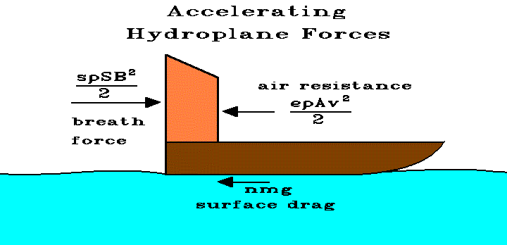
The acceleration of a hydroplane can be modeled using the general model for a powered vehicle if we assume a constant breath force. The equation of motion can be written grossly as blowing force, F, minus the resistance of the air on the sail, R, minus the sliding drag of the hull on the surface of the water,
ma = F - R - D
The force of friction due to sliding friction against a hydroplaning boat is caused by the weight, W, of the boat pushing down on the water surface. We write
D = nW where n is the sliding friction coefficient. The Weight, W, can also be written mg.
The force on the sail is that of pressure drag in reverse:
F = spSB2/2 where s is the pressure drag coefficient, p is the air density (air is being blown), S is the rearward cross-sectional area of the sail and B is the speed of the breath.
As the boat speeds up air resists the movement of the boat. The pressure drag is the same as for the sail force but the variables are renamed and the cross-section may be different.
R = epAv2/2 where e is the pressure drag coefficient, p is the air density (the boat is in the air now), A is the front cross-sectional area of the whole boat and v is the speed of the air which is the speed of the boat.
Putting these together with the signs of slowing force terms made negative we get:
Force = Sail Force - Frictional Forces
                       Air    Water
   ma =  spSB2/2   - epAv2/2 - nmg
We can now make the proper mapping between the physical factors of this model and those of the general one in the following table.
| General Model | This Model |
|---|---|
| F | spSB2/2 |
| M | m |
| Df | nmg |
| k | epA/2 |
| v0 | v0 |
| L | L |
| t | t |
Using this map we can apply the general model results to this specific model without having to derive the expressions all over again. Instead, the general model expressions are rewritten using the corresponding expression noted in the map table above. Then the expressions are simplified a bit to give the specific expressions we seek for this model. If any additional expressions are needed for this model, they are derived below.
The various factors above are related to one another using physical laws and analysis. Some of these relationships have special meaning in understanding the model. These as well as kinematic factors (like time, acceleration, speed and distance) are recorded in the next table as a summary of the model.
| Description | Units | Expression | |
|---|---|---|---|
| Equations of Motion | oz | ma = spSB2/2 - nmg - epAv2/2 | |
| Displacement Distance | in | Y = 2m/epA | |
| Initial Velocity | in/s | v0 = vc \[exp(-2(y-yc)/Y)-1] from coasting model v(y) | |
| Momentum Transfer | ozs/in | P = \[epA(spSB2-2nmg)]/2 | |
| Displacement Time | s | T = m/P | |
| Terminal Velocity | in/s | vt(B,n) = \[(spSB2-2nmg)/epA] | |
| Terminal Velocity | in/s | vt(y,t) = vt = Y arccosh(exp(y/Y))/t | |
| Warm-up Time | s | t0 = T arctanh(v0/vt) | |
| Warm-up Distance | in | y0 = - Y ln(\[1-v02/vt2]) | |
| Time | s | t(y) = T arccosh(exp((y+y0)/Y)) - t0 | |
| Velocity | in/s | v(y) = vt \[1-exp(-2(y+y0)/Y)] | |
| Velocity | in/s | v(t) = vt tanh((t+t0)/T) | |
| Distance | in | y(t) = Y ln(cosh((t+t0)/T)) - y0 | |
| Acceleration | in/s2 | a(t) = Y/T2cosh2((t+t0)/T) | |
| Breath Velocity | in/s | B(n) = \[(epAvt2+2nmg)/spS] | |
| Surface Drag Coefficient | scalar | n(B) = (spSB2-epAvt2)/2mg | |
| Hyperbolic tangent | scalar | tanh(u) = (exp(u)-exp(-u))/(exp(u)+exp(-u)) | |
| Hyperbolic arctangent | scalar | arctanh(x) = ln((1+x)/(1-x))/2 | |
| Hyperbolic cosine | scalar | cosh(u) = (exp(u)+exp(-u))/2 | |
| Hyperbolic arccosine | scalar | arccosh(x) = ln(x+\[xx-1]) |
Note: When modeling the first breath in a race, v0 = t0 = y0 = 0.
The easiest way to get B(n) is to start with terminal velocity,
vt = \[(spSB2-2nmg)/epA]
Isolate B2,
B2 = (epAvt2+2nmg)/spS
Take squareroots on both sides,
B(n) = \[(epAvt2+2nmg)/spS]
For the record, the sliding friction coefficient in terms of breath speed is found by solving the same terminal velocity expression for n,
n(B) = (spSB2 - epAvt2)/2mg
| [Next Section] | [Dry Dock] | [Title Page] |
| Raingutter Boat Racing - | Breathing Life Into Your Boat |
| Copyright © 1997, 2000, 2002, 2004 by Michael Lastufka, All rights reserved worldwide. | |