Dynamic Model of a Trikke T78 Air

Draft: 2 June 2020

Three mechanisms harnessed by riders and constrained by three cambering wheels fuel Trikke dynamics. Carving distinguishes the gait of a Trikke from most other body-powered vehicles. This undulating mechanism efficiently delivers 1) angular jetting and 2) linear pushing momentum from the rider to the Trikke. Centered below and behind the steering axis, the front guide-wheel of a Trikke articulates with the head joint, or yoke as a second-class lever. Within a fraction of a second while 3) turning it yanks the yoke into the turn transferring the trailer's angular momentum to the Trikke. A rapid turn with deep camber invokes this caster mechanism. Direct push and the more subdued involuntary castering feed into jetting, the most fundamental mechanism.

This study develops further the mathematical, dynamic Trikke locomotion model from a first principles perspective documented in the author's previous Body-Powered Trikke [Physics] article. The momentum transfer can be understood in terms of simple levers, rotations, inelastic collisions, and the Parallel Axis Theorem, all constrained by wheel friction. This effort expands the power production physics and geometry to propagation of local momenta and introduces a rider algorithm and rider scenarios modeled in a global frame. The result, a [calibrated], forward-feed, discrete Trikke dynamics computer simulation that provides many qualitative and quantitative insights into this elegant method of locomotion and exercise in investigated Trikke [behaviors].

An analysis by a daily Trikke rider

Technical sources for this effort include the Trikke patent applications, prior art patents, see [Trikke Patent], and two robotic control theory articles [RoboTrikke] and [Roller-Walker] written in 2005 and 2000, respectively. The patents assign credit for the main propulsion of the Trikke to "conservation of angular momentum", while the robotic papers attribute that role to castering; this author's designation for that phenomenon. While performing a "first principles" type of engineering analysis to derive equations suitable for simulation of the Trikke and rider experience, it became apparent that none of these sources had explored the whole picture. They seemed more interested in investigating the Trikke in the context of similarity to an atomic worm segment than as a rider-powered vehicle.

Rough Dimensions of a Trikke

In the patents, weak appeals to "conservation" arguments were made in a context where it was more important to distinguish the mechanical aspects of the invention rather than how a rider produces motion. Indeed, arguments concerning spinning ballerinas and arm positions are not satisfying and far from convincing. As acknowledged in the robotics articles, the Trikke is a nonholonomic system; one which involves constraints that are not conservative. In particular, a decrease in the turn radius does increase the angular acceleration by conservation of angular momentum, in the absence of friction. However, by the same conservation law, it is well known that this alone cannot add any angular momentum to the system as implied in the patents.

In the [RoboTrikke] project, a low-fidelity, ill-proportioned model Trikke was controlled robotically via castering with mixed results. Control equations grouped Trikke propulsion with that of the [Roller-Walker]. A second set of control equations simulated a token rider by "leaning" an elevated weight side-to-side across the two back wheels. An effect of this weak carving input was noted in their computer simulations, but was not attempted in the robot. However, the greater effects due to "jetting" and "slinging" the Trikke and rider's center of masses in opposite directions nearly parallel to the main axis was not addressed. Even the Roller-Walker should perform better using these modes of input, though it would be more difficult to coordinate than on a Trikke. In other work, the same authors show that a bike can carve [CarveABike] without peddling using a combination of carving-like motion and "balancing" to throw rider momentum along the path of the front wheel. The main issue was stability. A Trikke is intrinsically more stable.

In this present work, equations are derived describing the geometry and motion of the steering mechanism, the load moved by carving Extended-Trikke, the load moved by castering trailer and the wheels. A configurable digital robot model controls basic Trikke input without feedback. Equations expressing the local Trikke-Rider System (TRS) dynamics were previously derived by the author in a [physics] article and are implemented in the simulation. Trikke mechanical linkages allow the local frame to be embedded into the global, so that global placement and kinematics are addressed.

Program architecture is of little consequence to this descriptive effort. A simple simulation loop with a constant time step is all that is required to implement these models. There is no need for feedback or other control events. Better frameworks can likely be employed using Runge-Kutta algorithms, etc, but the results converge quite well without them.

A configuration file containing the detailed physical description of the Trikke, its subsystems, rider and simulation goals drives the simulation. Important internal and real-world measurable results are logged for each subsystem in the local Trikke coordinate frame and the global "lab" frame. Various forms of graphical or numerical analysis portray insights into the qualitative and quantitative data. Several behavioral scenarios are put forward including single input factor runs and coasting; the subject of the author's Trikke [behaviors] paper.

A Useful Model

A model becomes useful when it increases understanding that leads to better use, control or enjoyment of the target process or activity. A model often doesn't need to be measurably accurate to demonstrate differences that resolve questions, but must at least be qualitatively similar. By following physical and mathematical principles, it is posited that this model is at least qualitatively similar to a real Trikke. [Calibration] of simulated Trikke rides to real ones have brought the results of this model into the realm of reasonable quantitative accuracy.

Inputs to the Trikke model include:

  • the rider's mass, mR
  • the rider's steering angle limits, limθ
  • the rider's cambering angle limits, limγ
  • the rider's center of mass position limits, limψ and limψy
  • the rider's twist expressed around the Trikke's guide-wheel contact point, vσρ
  • the rider's steer/camber cycle time, τ
  • the time taken to turn the steering column (stem) to the other side, σ
  • a resting period between hemijets, φ
  • the TRS initial speed, V̅0
  • Trikke and rider solid models: the physical, geometric and dynamic properties of articulated parts
  • Environmental factors like acceleration of gravity, air density, etc..

Major components of the math and dynamic simulation model include:
  1. Quantified steering/cambering mechanism.
  2. Identification of constraints that turn steering and rider actions into motion.
  3. Construction and [calibration] of a friction model.
  4. Considerations for implementing the drive mechanisms presented in the [Physics] article.
  5. Propagation of local momenta constrained to the guide-wheel path.
  6. Injection of the local coordinate frame into the global.
  7. Creation of an automated rider to drive the simulated Trikke.
  8. Identification of categorical scenarios.
  9. Exploration of dynamic variables made possible by the simulation via graphics.
Some dynamic model design choices:
  • While solving for the contact point of the front wheel is inherently a 3-D proposition, only actions in the horizontal plane are considered for the Trikke frame. For example, there is a slight vertical displacement of the yoke when the front wheel is turned. While not difficult to compute, the resulting change in frame angle was not considered large enough to affect the dynamics significantly.
  • Body linkages (arms and legs) are not considered explicitly in the robot-rider model. 2-D input functions pattern steering, cambering, and the position of the rider's center of mass in a plane parallel to the road. However, because the rider's moment of inertia tensor changes with relative hand and foot placement, the motion of the handlebars and exact position of the foot decks are represented. Note, the rider's "twist" around his own center of mass is modeled. There is a "natural" twist due to pushing with the "outside" foot, which the rider can easily enhance with downward motion and hip action - see "jetting".
  • Wheel slippage is not considered. The contact "patch" is considered a point contact. Camber thrust is not computed. Rather than generally applying D'Alembert's principle to the wheel constraints and incorporating them into an equation of motion via "virtual work" or other technique, they are assumed in the formulation of the mathematical models, greatly simplifying the derivations and simulation.
  • A second-degree polynomial friction model was employed and [calibrated]. Though inclines and wind are not included in the model, the calibration study points to an elegant method for accomplishing this at a later time.

What is the model used for? Computer models give details of behaviors that are difficult or impossible to measure in real life. They are often used to compare the resulting behavior of subtle changes in parameters or sequences of inputs that would not be easy or economical to test for otherwise. In short, hypotheses can be tested and sometimes resolved that are not practical or possible to test in the real world.

Issues that can be addressed by models like this one, but not necessarily in this article, include:
  • How does a Trikke really work?
  • If castering contributes to Trikke locomotion, how much might it contribute?
  • Strategies (i.e., coordination of inputs) to produce the most drive impulse in different situations.
  • Assessment and comparison of field trial measurements with model results.
  • Can the Trikke be improved by changing its geometry?
  • Might some Trikke riders have physical characteristics that give them riding advantages?

There are many other avenues of possible exploration, including Design of Experiment DoE screening and modeling studies that can estimate the subtle advantages of various Trikke configurations and rider techniques.

Definitions

Simulation
A model constructed to demonstrate some aspect of a problem that typically encompasses familiar activities or properties of the model domain.
"All models are wrong, but some are useful." - [George Box], British statistician, 1976.

One reason this model of a Trikke might be wrong is because it is "simple". Details and physical processes that do not contribute to the more visible aspects of its dynamics are not addressed. Development and simulation of the model documented in this article are presented in the text at a conceptual level. Appendix A contains the detailed math and simulation models. Each has various parameters, independent and dependent variables which are defined in the pages where they are used.

Trikke Anatomy - What is a Trikke?

All body-powered Trikke vehicles consist of three long tubes attached to wheels with a shorter tube (handlebar) used to provide comfortable leverage for turning and cambering. The three main tubes articulate via a cambering joint, the yoke which constrains all three wheels to camber at about the same angle at the same time. The guide-wheel in front is mounted like a caster wheel with negative rake. Deceptively simple design. Pure genius. Synergistic engineering.

The model developed in this paper has been stripped down to a stick figure. Some of the illustrations, like the ones below, are based on a slightly more cosmetic, but mathematically precise [POV-Ray] version of the Trikke. Parts of the model are referred to by the names indicated in the image on the left in Figure 1. On the right, the main spans and articulations are illustrated in Figure 2.
Parts of a Trikke
Figure 1 - Parts of a Trikke
Main spans and articulations
Figure 2 - Main spans and articulations

Local Trikke Coordinate Frame (LCF) and Origin

Every model lives in some "domain". This one inhabits a 3-D mathematical world expressed via computer programs. Pseudo-code recipes express algorithms nicely where mathematical derivations are sometimes cumbersome. Expect to see some of both in the details.

Many vectors and coordinates in the model are measured in the local frame illustrated in Figure 3. This right-handed Trikke coordinate frame propagates local model effects to global behaviors.
  • x-axis, X̑: The forward direction of the Trikke is +x.
  • y-axis, Ŷ: The left side is +y.
  • z-axis: Z̑: Up is +z.
  • The "virtual" fork-arm intersection (yoke) of the Trikke is its origin point. This is the point where the steering axis and arm structures intersect virtually.
  • "Neutral" means the steering angle θ, and camber angle γ, are both 0-degrees; the "upright position".
  • The physical cambering mechanism separates the arms horizontally and vertically by a small amount so that they do not intersect when camber is non-zero. The simulated origin point remains at its virtual position on the steering axle regardless.
  • All measurements on the vehicle are taken relative to this yoke in the LCF - local coordinate frame of the Trikke.

Steering and Cambering

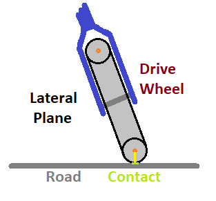
Figure 4 - Lateral Plane Guide-Wheel Contact

To simulate a trikke and rider system, the effect of the steering angle θ, and cambering angle γ, on the path of the guide-wheel must be known. Define the guide-wheel path ray with its origin at the wheel's contact point in a direction parallel to the intersection of the wheel's lateral plane with the road; see Figure 4. Locate the wheel's contact point by identifying the shortest vertical line from the minor radius of the toriodal wheel model to the road. In real life, the contact is a patch or a few of them if there is still a tread pattern on the wheels. Patches change geometry and deformation with turning and cambering that can affect the wheel path by torques and forces resulting in effects like camber thrust. Such patch properties are not a part of this model.

Tread Contact Points:

The tread contact points of the Trikke were measured in the neutral position. Structural points and the physical quantities needed to determine these positions from geometry were also measured. These included the articulation points needed to propagate changes in the Trikke's structure affecting the tread contact points as steering and camber are applied.

In the neutral position, the contact points (x, y, z) from the yoke origin in the local coordinate frame, LCF, are:

Table 1: Neutral Position Contact Points (inches)
Front contact σ = (3, 0, -14.81)
Right contact R = (-35, -10.375, -14.81)
Left contact L = (-35, 10.375, -14.81)

Note: the bridge symbol p͆ indicates a vector position measured from the origin of a coordinate frame, as opposed to an attached vector, r̚ (ray), or unattached vector, v̅.

To determine these contact points from the input steering angle, θ, and cambering angle, γ, in the local coordinate frame, a guide-wheel contact model was developed.

Trikke Guide-Wheel Contact
Figure 5 - Trikke Guide-Wheel Contact Patterns

On a Trikke, the guide-wheel axle is set behind the steering axis, a configuration called "positive trail". This causes the axle center to orbit the steering column in a circle when turned from -90° (turned to the right) to 90° (turned to the left). But the ground-projected image shown in the center of the figure is an ellipse with shortened height because the steering column is tilted toward the rider. The projection of the yoke falls to the brown dot at the crossing of the dark blue horizontal and vertical lines marked "0 in".

Each of the five turn plots project the turn pattern for each cambering angle γ set at -45°, -22.5°, 0, 22.5°, 45°. Their placement is the actual projection relative to yoke. Note tilting right, positive γ, projects to the left and vice versa. Each plot places a line from the axle center, represented by a dot, to the contact point on the tread. Twelve evenly distributed turn angles θ are represented between -90° and 90°. Light blue lines indicate θ < 0; red: θ = 0, blue: θ > 0. Note that on a physical Trikke, γ likely never exceeds +/-20° and once moving, θ stays between +/-30°. The values used here purposely exaggerate for a clearer graphic.

The distance between the wheel contact point (non-dot end of a line) and the yoke forms a lever that creates caster impulse described in more detail below. Initially, this lever points straight ahead 3-inches from yoke to the neutral contact point, the red dot on the center plot. If one only cambers to 22.5° (tilting the steering column to the right), the lever stretches almost 6-inches from yoke to the end of the red line on the plot to the left of center. Making the natural turn to the right increases its length even more.

In this model, the steering angle θ, camber angle γ, rider's center of mass ©R, and rider's jet velocity v̚σρ depend on time, t. These otherwise independent inputs are coordinated by the simulation to produce different "sweep" and driving patterns or strategies. Using the stem simulation model, any reasonable combination of θ and γ can be used to compute the corresponding tread contact point relative to the yoke in LCF. Table 2 illustrates one possible "sweep" cycle.

Table 2 - A Possible Sweep Cycle
Sweep CycleGuide-WheelContact Points (C͆F)
degreesdegreesinches from Yoke
γθxyz
25.00-90.005.4015.279-12.542
play animation or stop animation animation
Animation 1 - Trikke wheel sweep
20.83-75.005.376 5.030-12.936
16.67-60.005.005 4.751-13.391
12.50-45.004.359 4.159-13.892
8.33-30.003.673 3.108-14.360
4.17-15.003.178 1.661-14.692
-0.00 0.003.000 0.000-14.812
-4.17 15.003.178-1.661-14.692
-8.33 30.003.673-3.108-14.360
-12.50 45.004.359-4.159-13.892
-16.67 60.005.005-4.751-13.391
-20.83 75.005.376-5.030-12.936
25.00 90.005.401-5.279-12.542

The first two columns show an extreme sequence of γ and θ for one complete sweep cycle. The next three columns are the local coordinates of the contact point beneath the yoke. These contact points are rarely in the middle; y = 0. They are also higher than the neutral contact point at -14.812 z. This indicates that the Trikke tilts forward a bit (Td) at the left and right edges of each sweep. Yoke is held constant in the animation at world coordinates (0.0.0) and a shadow helps emphasize the height gap of more than an inch and a half from the ground.

The rear wheels of a Trikke do not steer, but camber at the same angle as the guide-wheel. The steering model used with θ = 0 produces the rise and fall of the rear wheel contact points due to cambering alone. In the animation, the rear wheels are kept on the ground (not shown) so the ground rises and falls by the amount dictated by cambering. The sweep shown in the animation is not the same as that in the table; both are for illustrative purposes only.


Drive Generation

A body-powered Trikke is driven by a virtual second-degree lever as elucidated in Trikke [Physics]. Riders control the free end of the lever via the handlebars of the steering column and forward forces they intentionally generate by shifting their body's center of mass and rotating into the guide-wheel path. Changes in stem angles alter the guide-wheel path and the magic lever's turn-radius, which vary the forward leverage on the TRS center of mass to carve. These same stem angle changes alter the triangle between the guide-wheel contact, the yoke and the transom, producing small, forward caster impulses.

Impulses are changes in momentum, due to applying a force over time. The force typically starts out stronger and then tails off. It acts vigorously over a very short period of time - fractions of a second. Expending a particular amount of energy in a shorter time, the greater the force and impulse it creates - the greater the change in momentum. When the mass of a system remains the same during its operation, then momentum can be thought of as velocity, v̅, and impulse as change in velocity, Δv̅ (as in orbital mechanics). The greater the impulse, the greater the Δv̅ and therefore the greater v becomes! Many people find the trikke difficult to learn because they do not grasp how to produce a coordinated sequence of periodic motions that drive the Trikke. This is understandable, the movements can be quite subtle to the casual observer.

Simulated Trikke Components

Simulated agents produce locomotion by their dynamic actions with each other. Impulses, momentum transfer, forces, rotation all have a source agent and recipient agent according to Newton's 2nd Law. Something pushes and something else gets pushed. Something pulls, something else gets pulled. Generally, both rotation and translation result depending on the relationships of the force vectors and the agents' centers of mass. See Vector Decomposition in Appendix C for an illustration. The Trikke has two pairs of reaction agents that are not totally independent.

Each of these main components is broken into subparts. The subparts are also broken down. Eventually, "irreducible" parts make up the subparts. In this simulation these are shaped like cylinders and blocks. Each has mass, a center of mass, position, moment of inertia tensor, geometry and a few other properties necessary to build up a dynamic picture of what is happening to them. By composing the properties from irreducible to main component, the credibility of the geometry and physics is maintained in the "solid" models in the usual ways.

  1. The Steering Column, or stem, is the first of 3 simulated components that has a profound effect on the locomotion of the Trikke. Most importantly, the stem wheel guides the Trikke, channeling all of its momentum into the trajectory of that wheel. It also creates two weak impulses. When the guide-wheel turns from a non-zero steering angle toward 0° then past it, castering first pulls the trailing frame and rider into the turn giving them angular momentum. As the turn completes, it is released in a weak jet. Parts of the rider - hands and wrists - are essentially part of this extended steering column.
  2. The second component of the model is the afore mentioned Trailer. It is composed of the parts of the Trikke and rider that get rotated and pulled by the castering action of the steering column; Caster-Pull. The remaining parts (steering column with its guide-wheel, rider's hands and part of the forearms) are pushed slightly forward via the trailer by the second impulse generated by the steering column, the Caster-Push.
  3. Component number three compliments the motive mass of the rider in carving. Part of the rider's mass travels with the Trikke, while the remainder moves quickly in the opposite direction. Parting the two centers of mass slings the Trikke along the guide-wheel path. The compliment of the rider's motive mass is the Extended-Trikke. It is composed of all of the parts of the Trikke and those of the rider that are essentially stationary with respect to the Trikke. This is the part of the TRS that gets slung forward when the rider quickly shifts his center of mass backward into the turn resulting in a Direct-Push.
  4. The rider's body core is the fourth component. Most of the rider's body participates in slinging the Extended-Trikke. Hands, feet, part of the forearms and lower leg do not contribute their mass to slinging. Rather they get slung, and are thus considered part of the Extended-Trikke.

These components and their dynamic interactions produce the Trikke locomotion drive actions. They are presented in the Trikke [Physics] article. These drive interactions include:

  • Jetting (rider's intentional rotation in carving)
  • Direct-Push (rider's intentional forward sling and latteral lean in carving)
  • Caster-Pull and Push (frame linkage's response to turning and cambering)
Summary of Equations Implemented from the Trikke [Physics] Article.

Jetting

All of the drive mechanisms feed into the jetting mechanism by imparting a local velocity to the guide-wheel along its path. In particular, the rider generates a direct rotation input, "jetting" or more precisely, "hemijetting" since half of the jet is performed in half of a drive-cycle.

The main result of the Trikke Hemijet Model represents the local instantaneous velocity, v̚ of the Trikke-Rider System center of mass. A local velocity imparted to the guide-wheel along its path, v̚σρ generated by some agent like the rider's rotation or resulting from a direct push or from the caster mechanism is the main input to the model. Others provide geometric context: r̚σ, the radius-ray from the turn-center to the guide-wheel contact point and r̚, the the radius-ray from the turn-center to the TRS center of mass.

eqn jp4: v̚ = (ȓσ × v̚σρ) × r̚/rσ

Direct Push-Pull

Determination of v̚σρ, the local velocity to the guide-wheel along its path generated by a direct push from the rider on the handlebars is provided by the Trikke Direct Push-Pull Model.

The main input to this model is the rider's change in center of mass ©͆R position. It is limited by the foot decks on the arms of the Trikke and the position of the handlebars. When the rider's position changes, the resulting momentum splits into orbital and radial components. The orbital component produces a driving jet impulse, while the radial component reinforces wheel constraints via friction. This momentum has mass mR and veloctiy v̚R. ρ̑σ is the guide-wheel path unit vector. M, represents the TRS mass constrained to travel in the direction ρ̑Trs.

Note when v̚R · ρ̑σ > 0, the rider is pushing into the guide-wheel path. When v̚R · ρ̑σ < 0, the rider is pulling.

eqn dp6: v̚ρσ = - mR (∂©͆R/∂t · ρ̑σ) ρ̑σ/(M ρ̑Trs · ρ̑σ)

This locally generated velocity is treated as the input to the jet model to find its contribution to v̚ at the TRS center of mass.

Caster Pull-Push

The relative motion of the guide-wheel contact point, the yoke and the trailer lead to a small jet rotation. Castering is initiated by the side-ways motion of the yoke as the result of a turn. The Caster Push-Pull model provides the jet velocity v̚σρ that is transformed by the Trikke Hemijet Model into v̚; the contribution of castering to the TRS center of mass velocity.

Jet velocity from castering depends on the movement of the yoke into the turn and the rider's proximity to the handlebars. The faster the turn; the stronger the jet. A rider close to the transomp isn't thrown into the turn as much as one close to the handlebars, but a quick turn becomes easier to perform. As the rider and trailing arms are rotated into the turn over a time Δt with mass mt, moment of inertia It and center of mass ©͆t by the Trailer-Lever with fulcrum at the contact point C͆σ, they build up angular momentum. As the turn slows, this momentum releases via the contact point in direction ρ̑σ to the TRS with mass M constrained to orbit the path ρ̑Trs.

eqn cp10: v̚σρ = -(It + mt (T̑p - ©͆t)2) ((T̑p × (C͆σ' - C͆σ)/(Tp Δt)) - (T̑p' × (C͆σ" - C͆σ')/(Tp' Δt'))) × (T͆p - C͆σ) × ρ̑σ × ρ̑σ/(M ρ̑Trs · ρ̑σ)

This locally generated velocity is treated as input to the jet model to find its contribution to v̚ at the TRS center of mass.

Using velocities in the Simulation

Because the approach to the physics of a trikke is mostly through momentum considerations, the results summarized above are instantaneous velocities. To use them in a discrete or time-sliced simulation requires some estimates based on the velocities calculated at each time-step. Appendix C presents the details for these estimates in Δv for Simulation.

2nd-Degree Polynomial Friction Model

Generally, friction is modeled as:

eq 1: F = -μ Λ

where F is the friction force in Newtons; μ is a scalar (unitless) friction coefficient; and Λ is the load on the interface in Newtons.

Often, μ is a function of the velocity at the interface. For dry interfaces, μ might be modeled as a constant a. With bearings, the model may include a direct velocity component multiplied by a coefficient b. Wind and other fluids operating on the interface often introduce a v2 dependence scaled via a coefficient c.

In a separate empirical study [calibrated], the author determined the following friction model for his T-78 Air Deluxe; eq 2. It is used in the simulation to make the model's kinematic results quantitatively match those of his Trikke. The friction model coefficients may be different for other Trikkes, but they should all have the same basic characteristics and ranges similar to those shown in Figure 7 below.

eq 2: μ = 0.14968462 - 0.13434041 v + 0.03134038 v2
Friction Model Graph
Figure 7: Friction Model Graph

When the author goes for a ride, the combined load on the wheels is about 81 kg. Since it is different for others, this graph shows the friction coefficient μ instead of the force. At 0 velocity, the initial force that he must supply is about 26.75 lb (119 N). Because the coefficient of v is negative in eq 2, it gets easier to propel the Trikke until about 5 mph (2.25 m/s) where it takes very little effort at all, a so-called "sweet spot". The green area represents speeds at which it is as easy or easier to keep the trikke accelerating as it is to get it going.

Exercise: Imagine catching an 8.8-pound dog (like a large Toy Poodle, 4 kg) dropped from 3 feet in the air and bring it to rest after contact in about a foot. That means you bring the dog to a halt in about one-third of a second. This dog imparts an average of 8.8 lb (40 N) of force to you over this short time, which means the initial contact force was about 26.75 lb. The contact force decreases rapidly as you bring it to a halt still feeling its 8.8 pound weight and there are no injuries - just one nervous pet. If you just have cats or no pets of the right size, consider using a 10-pound medicine ball instead; they can be a tidy 8 inches in diameter and won't claw.

Past about 9.5 mph (4.25 m/s), the graph shows that it takes more and more motive force than initially to sustain greater velocities on the Trikke. Beyond about 10 mph (4.5 m/s), extra input force yields less and less increase in velocity until the rider can go no faster; "terminal velocity" has been reached.

This one-dimensional friction model is easily extended to three, where the mass, m, is that of the load supported by the wheels and the vectors align with the path of each wheel to which it is applied.

eq 3: F̅ = -(0.14968462 - 0.13434041 |v̅| + 0.03134038 v̅· v̅) m g ρ̚

Strictly speaking, eq 3 is not a completely accurate way to implement this friction model. The main speed-limiting term in v̅· v̅ applies more to the "whetted" frontal area of the entire Trikke than to individual wheel fluid dynamics. It was nevertheless implemented this way to keep the model simple. Also, the resistance due to wheel spin-up and assistance due to spin down, (i.e., wheel inertia), is separately estimated in this computer model, and is actually confounded in the velocity dependent term of this empirical friction model.

Adding torques as in eq 4 created by the friction force at each wheel factors into finding the center of mass friction force in eq 5. Note, r̚w is the turn-ray to each wheel contact point with w in the index set {σ i r} for the stem, left and right wheel. Likewise F̚w represents each wheel's friction.

eq 4: τ̚ = r̚σ × F̚σ + r̚l × F̚l + r̚r × F̚r

The friction force at each wheel is solved via inverting the cross-product for total torque of the force F̚© at the center of mass ©͆ around the turn-ray r̚ from the turn-center T͆c to ©͆.

eq 5: F̚© = τ̚ × ȓ/r
Wheel Stride
Figure 8: Wheel Stride

Each wheel, w, has a slightly different velocity vector, v̚w, because a Trikke rarely travels a straight line. Δv̚w, the difference in wheel velocity from the Trikke's center of mass velocity is stride. The physical and geometrical derivation for stride is in Appendix A. Each wheel has a different stride, so the friction that opposes it is different. Because wheel friction follows each wheel's orbital path, the sum of friction magnitude over all the wheels is not equal to that calculated at the TRS center of mass, cm. The load on each wheel also causes differences in friction.

Note, the diagram on the left in Figure 8 is constrained to travel around the turn-center, T͆c. That on the right is free to rotate as if on ice or other low or no friction surface. Radials, r̚i where i stands in for {T σ L R}, on the left are scalar lengths at right angles to the wheel paths through the instantaneous turn-center, T͆c. The radials on the right are rays to the TRS center of mass forming various angles to the wheel path directions, ρ̑. The velocity differences, Δv̚i, will generally be smaller for the constrained vehicle. Rotation, ω̚, around the TRS center of mass is the same as that around the turn-center, but the radial lengths are shorter. Friction constrains the Trikke to operate according to the diagram on the left.

When the Trikke is turning, the velocities of its parts are proportional to the ratio of those part's turn-rays to the center of mass with faster parts having longer turn-rays. In the simulation, the TRS velocity is changed by the ratio of the turn-rays of the guide-wheel velocity origin and the TRS center of mass. Each wheel's friction depends on its stride, load, and path unit vector, but also its turn-ray ratio when applied to the TRS center of mass. See the center of mass and friction derivations in Appendix A for details.

Trikke Path Propagation

Once the simulated Trikke has a velocity, a propagation model determines where the Trikke goes. Just like the constraints on impulse production, there are constraints on the path it can take. These constraints involve linear and angular momentum and wheel friction. Computing a local path step is not enough. So far, Trikke model discussion has focused on a local coordinate frame, LCF. Now, a Global Coordinate Frame, GCF, is needed. The LCF is embedded in the GCF by the position of the yoke in the GCF and the angle, λ, between the x-axis of the GCF and the x-axis of the LCF.

Path Propagation

There are many sources from which changes in momentum arise. Since part mass is constant, velocity deltas of the TRS center of mass are used instead of changes in momentum (impulses). Delta velocities arise from carving, castering, friction and wheel inertia. The last source is bound up with the wheel's velocity and is confounded with the velocity dependent component of friction in the empirical friction model. The simulation computes this contribution, but does not apply it to the path velocity. Moment of inertia is calculated for each wheel. A Trikke is affected by wheel inertia the same way as other wheeled vehicles - as a change in mass; so called "inertial mass". For a Trikke the ratio of maximum inertial mass to TRS mass is less than one-percent.

The total momentum from the last simulated step i was M v̚i and is now M (v̚i + Δv̚) where all the impulses and friction have been reduced to their contributions to Δv̚ at the TRS center of mass.

Path Propagation

Having determined the center of mass path unit vector and TRS center of mass velocity, the simulation propagates the Trikke's next path step and guide-wheel contact position. Dead-reckoning applies to the step when the Trikke travels a straight line. But most of the time, the Trikke orbits a turn-center with a radius shrinking from infinity to a couple of feet and back again. The current kinematic state determines the turn-center, but ends the step with a new one. See the equations and other details for pathing in Appendix A.

Thus, the sequence of guide-wheel contact points traces a smooth curve (like the green arrow in Figure 9), less often a line. Over a very short interval of time, Δt, like 1/100th of a second, steering and cambering produce a curve with a turn-centerc at the intersection of a line between the rear wheel axles and a line parallel to the guide-wheel axle as seen in some of the diagrams like Figure 8. This estimate does not account for wheel slip or camber thrust that can affect all wheels since they all camber together at the same angle. During Δt, the steering angle changes from θ to θ', the camber angle from γ to γ' and TRS velocity from v̚σρ to v̚σρ'. These cause other quantities to change, like the yoke position from which the location of the guide-wheel contact point C͆σ is found in the GCF. Friction constraints allow only the velocity component perpendicular to the turn-radius r̚σ (along unit ρ̑ ) to propagate the step; momentum in other directions dissipate in friction.

This, "Δt step" reflects

  • the total momentum of the Trikke and rider
  • carving impulse from the rider
  • caster impulse from changes in steering and cambering by the rider
  • mechanical tread friction, bearing friction, wheel inertia, air resistance, etc., via the friction model.

Knowing the initial turn-center T͆c, turn-ray r̚σ, jet velocity along the guide-wheel path v̚σρ and Δt, the step s̚ at right angles to this turn-ray is calculated with the magnitude of the jet velocity multiplied by this delta time. Note that this approximation is "flat" not an arc distance (green arrow). The simulation computes the angle spanned by the step s̚, which "rounds" the arch. The LCF also turns through this angle Δλ. A new turn-ray r̚σ' fitting with the end of the step, steering θ' and cambering γ' angles is calculated. From the new contact point and LCF orientation, the new global location of the yoke (LCF origin) is found, so that the new LCF is ready to locate the rest of the Trikke and rider.

Placement

Placement into GCF

Figure 10 zooms in on the upper left portion of Figure 9. The geometry of the Trikke depends on the steering angle θ, and camber γ. Particularly, the relationship between the guide-wheel contact point C͆σ' and the Yoke'. In particular, the centerline Ȼ angle relative to the contact point path is known. Once the new guide-wheel contact point, Cσ', and the amount of rotation caused by the step s̚, are known so is the new angle, Δλ+λ, between GCF and LCF. Δλ is the angle between the old local x-axis in the global frame (light blue ray) and the new local x-axis in the global frame (blue ray).

With the new LCF rotated to the global frame, all of the Trikke wheel contact points, can be translated to global coordinates. Note the geometric placement relationships in Figure 10 and derived in Appendix A.

Digital Robot

Controlling a Trikke Simulation requires a time sequence of coordinated commands emulating a basic understanding of how a human rider controls a real Trikke. A single iteration step of the simulation can determine responses to impulses in various Trikke configurations. But for sustained travel, the following goals were implemented:

  • Periodic execution of control protocol.
  • Control variables within human operating ranges.
  • Limits of control and important internal variables become robot controlled inputs.

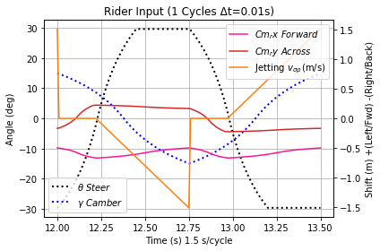
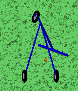
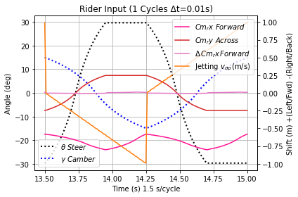
Turns out, for the purposes of exploring a Trikke's dynamics and kinematics, a feed-forward control system is all that is required. No feedback, state filters, control laws, governors, AI or goal chaining need be developed. Riding a Trikke feels simple, natural and magic because it is. Even a digital robot savant can do it. This robot implements a "bow tie-shaped" trajectory for its virtual center of mass (see Image 20 below) coordinated with steering, cambering and jetting rotation. Each control input is periodic over a set of limits. One such configuration is plotted over 3 cycles in Figure 11. Not everyone drives a Trikke this way; other drive-cycles are possible, even with this robot. It is not necessarily optimal, but it is simple.

Robot Input / Output

Trikke riding digital robot input includes:

  • Current phase: in the normalized, unitless range [0,1) which represents the time interval from 0 to τ, the drive-cycle period or cycle-time in seconds.
  • θ: Steering angle limit: to the left(+) and to the right(-). The robot sweeps from -θ to +θ each cycle.
  • γ: Cambering angle limit: to the left(-) and to the right(+). The robot sweeps from +γ to -γ each cycle.
  • ψ͆x(2): Rider's center of mass limit relative to Yoke: Each cycle, the robot slings from ψ͆x1 to ψ͆x2 and then back again on the x-axis.
  • ψ͆y(2): Rider's center of mass limits relative to the centerline: to the left(+) and to the right(-). Each cycle, the robot leans from ψ͆y1 to ψ͆y2 and then back again on the y-axis.
  • aσρ: Rider's constant jet-acceleration in m/s2. Starting at σ/2, jet velocity ramps up from 0 in steps of aσρ each time-step left in the half-cycle.
  • σ: Phase interval during which θ steers from one limit to the other. Range 0 to 0.5 cycles.
  • φ: Phase interval during which the robot rests. Range 0 to 0.5 - σ cycles.

Note that Cycle time τ, Mass of the robot-rider w and TRS initial velocity v0 are simulation imputs, but not robot input.

Initially, the limits of steering, cambering, rider center of mass, jet-acceleration constant, turn quickness and rest are set by the calling program. Drive period τ is normalized between 0 and 1, with the simulation controlling the current cycle phase via that range. Note, time is not a direct input. It is indirect via cycle phase. A drive-cycle consists of two half-cycles, one turning and/or cambering to the left, the other to the right. Phase between 0 and 0.5 turns to the left, while 0.5 to 1 turns back to the right. The first cycle begins with the guide-wheel steering and camber at the average of the specified limits. Subsequent cycles begin where the last one left off.

Notice the rider's intentional twist around their center of mass is modeled as the jet-acceleration constant. If the rider does not jet, there is still a bit of natural twist. To not twist at all, the simulation would have to apply the parallel axis theorem for angular momentum to reduce the system's rotation. By ignoring the natural twist, the robot is actually twisting enough to have no effect on the rotation; no jet. Additional rider's twist is input as the jet-acceleration constant. Each half-cycle, jet-acceleration ramps the jet velocity linearly from zero to (0.5 - σ/2 - φ) aσρ. The center of mass is self-calibrating, as it cannot exceed the bounds of the Trikke trailer or the Trikke would become unstable. Jet is not so limited and it is not known how much a rider can muster.

Robot output includes:

  • θi: Instantaneous Steering Angle
  • γi: Instantaneous Cambering Angle
  • ψ͆i: Instantaneous Rider Center of Mass position vector relative to Yoke
  • vσρ: Instantaneous Rider generated jet-speed reckoned at the guide-wheel contact point

Most parameters employ a horizontal sigmoid transition between the specified limits within their phase in the cycle. Figure 11 below shows robot model output logged for the last cycle of a typical simulation run. Only the first cycle starts out different with θ and γ set to 0.

Typical Simulation Input Configuration:
θ = 30°, γ = 15°, ψx = (-0.5 -0.675) m, ψy = (-0.25 0.25) m, vσρ = 2 m/s2, v0 = 0 m/s, τ = 1.5 s, σ = 0.3 cycles, φ = 0, w = 70 kg

Figure 11 - Robot Output
play animation or stop animation
animation
Animation 2 -
Robot Center of Mass

Drive Control Scenarios

Some example robot drive control scenarios are presented below. Most would be very difficult for a rider to perform in real life. Most do not result in viable forward movement. Initial velocity, v0 is a simulation configuration parameter that starts the Trikke at time 0 with the provided velocity. When robot inputs are given as a single limit value, it means the limits are - and + that value or where there is a natural minimum, the limits are min and value. ψx has such a minimum value at -0.5 m. In addition to the physical Trikke parameters, other simulation configuration parameters include things like a time-step increment and options pertaining to simulation termination.

Table 5 - A Few Drive Control Scenario Examples
Scenarioθ
(°)
γ
(°)
ψx (m)ψy (m)vσρ (m/s)v0
(m/s)
Coast00-0.5004
Turn Coast15*0-0.5004
Steer Only450-0.5000
Camber Only015-0.5000
Caster Only4515-0.5000
Sling Only00-0.675000
Lean Only00-0.50.2500
Jet Only00-0.5020
Push Only00-0.6750.2500
Carve Only00-0.6750.2520
Steer Carve300-0.6750.2520
Camber Carve015-0.6750.2520
Caster Push3015-0.6750.2500
Caster Jet3015-0.5020
Caster Carve3015-0.6750.2520
Caster Carve Cruise3015-0.6750.2522.2

* Unlike the usual limits sweep, once turned to this angle, steering is frozen. Both limits are set to the same value.

Graphic Output

Many of the simulation result plot types appear in the following pages. Their purpose is not an explanation of the typical carving run they portray, but to indicate what is produced by the simulation. Interpretation of the results of various simulated scenarios is the subject of Trikke Behaviors.

The following indicates how some output quantities were converted for display in the plots below.

Energy from velocity
For an output velocity v, its kinetic energy is K = M v2/2 where M is the appropriate mass.
Energy from change in position
Changes in position occur over the simulated time interval Δt. Treat the change as a velocity: K = M (Δx/Δt)2 where M is the appropriate mass.
Work from force
Starting with an output force like friction, its work is W = F λ where λ is the distance traveled in a simulated time interval Δt. The Work Energy Theorem allows work to be equated to and compared with quantities represented as energy.
Acceleration from velocity
Estimate using the interval definition for acceleration: Ɑ = (vi - vi-1)/Δt
Color Coding
Color is used to indicate different, but related quantities in a chart. For example, in energy profiles, reddish curves portray dissipations, while greenish ones represent contributions to locomotion.
Cycles
The number of cycles covered by the plot are shown in the title. Only one cycle is needed to chart quantities with cycle patterns that don't change. Other plots run for the number of cycles needed to show a behavior pattern or reach terminal velocity or to stop.
Table 6. - Graphic Output

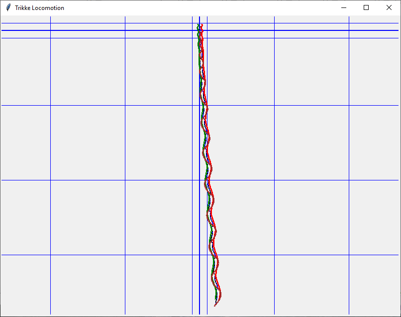
Image 1. - Wheel and Cm Tracks

Full track shown. One meter between smaller spaces between lines; 10 meters between the larger spaces.

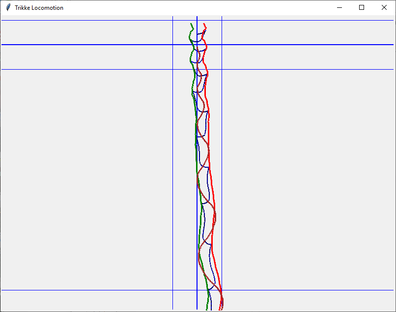
Image 2. - Magnified Tracks

Track color codes: Brown - guide-wheel; Green - right wheel; Red - left wheel; Blue TRS center of mass.

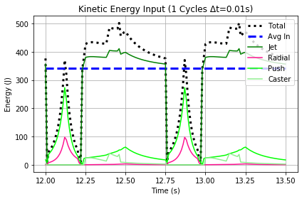
Image 3. - Input Energy

Compares energy input components over the trial. Robot input is static each cycle. The blue line is the average.

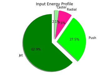
Image 4. - Input Energy Profile

Compares energy input components. Some of this energy like rider recoil helps generate components that directly affect locomotion like direct Trikke push.

Image 5. - Rider's Control Input Pattern

Robot steering, cambering, two dimensions of center of mass displacement and jetting on one plot. Note two vertical axes.

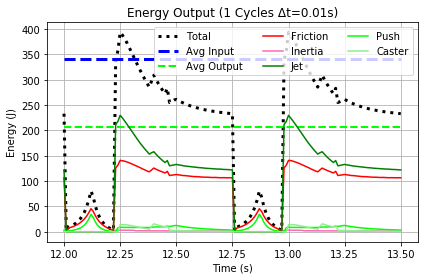
Image 6. - Output Energy

Compares energy output and expenditure components. Friction is measured as work. Average input slightly above average output demonstrats most energy is accounted for.

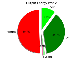
Image 7. - Output Energy Profile

This pie serves up the major contributors to total energy output. For efficiency, add the greenish parts together. The reddish ones are "wasted".

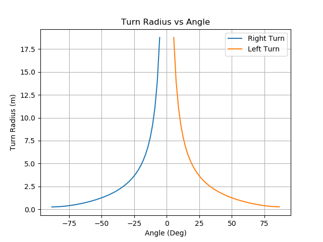
Image 8. - Turn Radius Vs. Turn Angle

The turn radius depends only on the steering angle. Turn radius is infinite at 0 x.

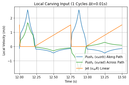
Image 9. - Carving Input

Effective change in guide-wheel velocity for the rider's jetting and direct-push.

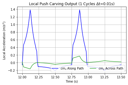
Image 10. - Carving Output

Change in TRS cm velocity along (blue) and across (orange) path due to Direct-Push.

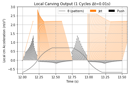
Image 11. - Carving Output Vectors

Vectors showing direction and relative size of jetting (orange) vs push (black) velocities at TRS cm. Notice how straight forward they are!

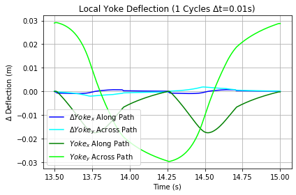
Image 12. - Local Yoke Deflection

Yoke position and deflection over a cycle. This drives the separation producing caster effects.

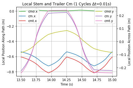
Image 13. - Local Stem and Trailer CM

Center of mass positions for the stem, TRS and trailer that participate in castering effects.

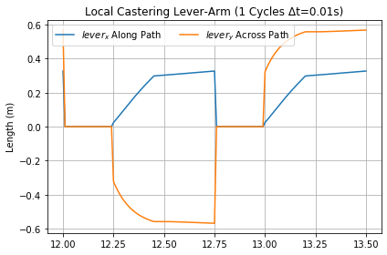
Image 14. - Castering Lever-Arm

Castering dumps the trailer's orbital momentum into a jet via this lever-arm. X (blue) and y (orange) components are shown.

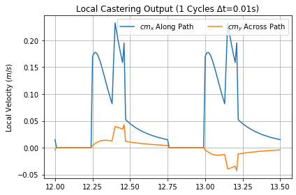
Image 15. - Castering Velocity Output

Velocity at the TRS center of mass along the path (blue) and across it (orange).

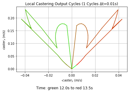
Image 16. - Castering Output Hodograph

Contribution of castering to TRS cm velocity. Along and across path components plotted against eachother. Abscissa is reversed.

Image 17. - Castering Output Vectors

Velocity vectors (orange) at the TRS center of mass synchronized with guide-wheel path vectors (brown) due to castering.

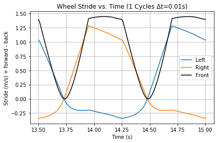
Image 18. - Wheel Stride

Stride along each wheel's path. Highest on the outside of the turn. Inside stride is slightly negative.

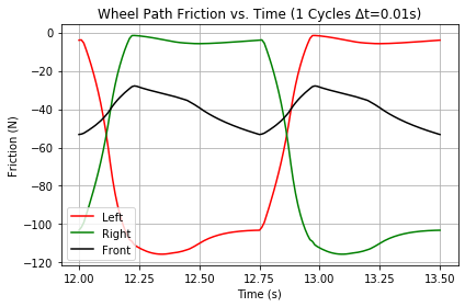
Image 19. - Wheel Friction Along Path

Friction along each wheel's path. Most detracting on the inside of a turn as the rider shifts weight that way. Most weight on trailing wheels.

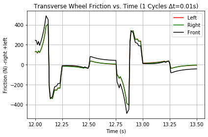
Image 20. - Wheel Friction Across Path

This friction enforces the "travel in an arc" constraints.

Image 21. - Local Rider Cm Hodograph

The rider's "dance". Rider's center of mass position over a cycle.

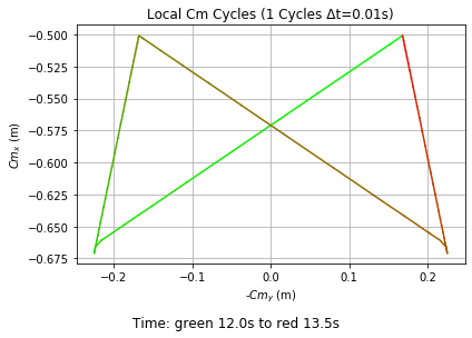
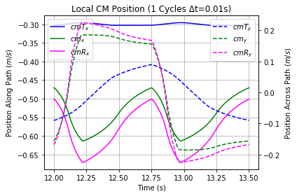
Image 22. - Local Cm Position

CmT: Trikke center; Cm: TRS center; CmR: Rider center. Along the TRS center of mass path and across it.

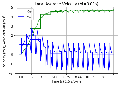
Image 23. - Local Velocity and Acceleration

Instantaneous and average TRS trajectory velocity and acceleration from stop to terminal velocity.

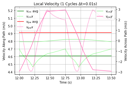
Image 24. - Local Velocity

Velocity along and across their respective path vectors for TRS center of mass and the guide-wheel contact point.

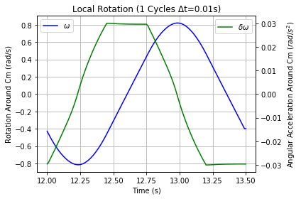
Image 25. - Local Rotation

Rotation around the TRS center of mass over a cycle. ω should be symmetric around zero, but is offset due to integration of deltas beginning away from a zero-crossing each cycle.

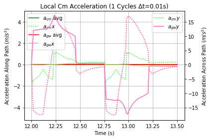
Image 26. - Local Acceleration

Acceleration along and across their respective path vectors for TRS center of mass and the guide-wheel contact point.

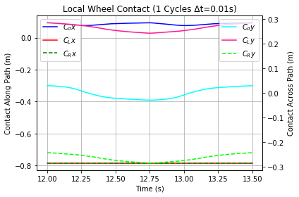
Image 27. - Local Wheel Contact

Position of the wheel contact points wrt. the yoke, x-axis (along) and y-axis (across).

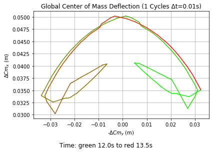
Image 28. - TRS Cm Deflection Hodograph

Figure traced by changes in the TRS cm in the Global frame.

Conclusion

A calibrated dynamic Trikke simulation was developed implementing drive dynamics from a paper by this author based on first principles of [Physics], vector analysis and rider experience. Four assembly models of the Trikke-Rider System decomposed the system; steering mechanism, trailer, extended Trikke and the robot-rider. A friction model and calibration method was developed and documented in another paper. The rider was modeled as an autonomous state machine providing reasonable input to the Trikke. Sets of prototypical velocity generation parameters yielded illustrated Trikke locomotion responses. Other aspects of Trikke geometry, physics and useful mathematics are derived in the appendices below.

Some parts of the simulation are briefly documented here and used extensively in the simulation [behaviors] paper including many charts and graphs of the dynamics and kinematics of various Trikke simulation scenarios. Some show paths carved out by the Trikke under various driving scenarios, while others compare internal dynamic and kinematic variables like friction forces and velocities. One of the more interesting chart types is the "energy profile" showing how much energy is directed into or out of the various mechanisms of the Trikke model as a percentage of the total energy input by the robot or output by the system.

It is hopped this simulation and ride analyses based on the simulation will elucidate the [magic] of the ride for many readers. Riders may gain insight to improve their sport. Non-riders might be able to appreciate the synergism in its engineering and begin to understand how they too can ride a Trikke. Naturally, the best way to digest what is written here is to go for a ride!

Appendix A: Model Derivations

Parameters of the Trikke Model

The math and simulation models are based on the following model parameters. Parameters define a simulation configuration. They do not change during a simulation run, but can change between them. Many were measured from a Trikke T78 Air Deluxe. These are mostly independent variables describing the geometry and physical characteristics of the Trikke. Each symbol may be modified in the following ways, but not all modifications are relevant for every symbol.

  • : No modification carries the "usual" or default definition for a symbol. Usually this designates a scalar or a scalar based on a vector (such as v = ║v̅║ designates the L2 norm of a vector; its length). Some non-roman symbols are designated as vectors in the following tables.
  • ̅: An elevated long bar designates a "free" vector interpretation for the symbol. Usually written component-wise v̅ = <x y z> or <vx vy vz>. Note the use of angle brackets and spaces rather than commas.
  • ̑: A circumflex designates a unit vector of the "free" vector interpretation for the symbol; v̑ satisfies 1 = ║<x y z>║
  • ͆: An elevated "bridge" designates a "coordinate" interpretation for the symbol. Usually written component-wise as v͆ = [x y z] or x X̑ + y Ŷ + z Z̑ using the basis vectors of some designated coordinate frame <X̑ Ŷ Z̑>, global, local (Trikke with origin at Yoke) or some part frame. Note the use of square brackets. A "free" vector is based in a coordinate frame as well, but the x y z components carry other assigned meanings; they are not coordinates of any of these frames.
  • ̚: Emphasizes a vector's use as a ray. The symbol is called an elevated "left angle". Rays have an origin and a direction. The origin is understood in context. Example: let v̚ = <x y z> at a position p͆ = [px py pz]. Its free vector is v̅ = <x y z> and end position is v͆ = p͆ + v̚ = [px+x py+y pz+z]. This definition is consistent with position vectors, which all start at an origin [0 0 0]. Many vectors including acceleration, Ɑ̅, and velocity, V̅, are actually rays since they are based at a point like the center of mass, ©, but we all got used to them being considered free vectors in school!
  • min[sym] : When prefixed by "min" the quantity designates a lower limit for the value of the symbol. Example: minθ = -90 degrees.
  • max[sym] : When prefixed by "max" the quantity designates an upper limit for the value of the symbol. Example: maxθ = 90 degrees
  • lim[sym] : When prefixed by "lim" the quantity designates a limit for the values of the symbol. When the symbol is a scalar, lim designates a minimum and a maximum value. limθ = [minθ maxθ] = [-90 90]. A vector lim designates some extreme vector or coordinate value defined in context or limits on one of the components which is made clear in context.
  • [sym]x [sym]y [sym]z: Designates a component of the vector symbol. v̅ has components x, y, z or better, using the symbol, vx, vy, vz.
  • [sym]0: Designates an original or starting value for the symbol in context.
Symbol Value Description
[0, 0, 0] Origin of the local coordinate frame (LCF) of a Trikke. The virtual intersection of the steering column and wheel-arms where the cambering head-joint is located. All LCF point measurements are made from this reference point.
M 81.3 kg Total mass of the simulated Trikke and Rider. Units kg.
m(T t E aL aR σ w h R) mT = 11.22 kg
mt = 77.48 kg
mE = 21.72 kg
maL = maR = 3.74 kg
mσ = 3.74 kg
mw = 0.74 kg
mh = 0.46 kg
mw - mh = 0.283 kg
mR = 70 kg
Mass of the object indicated in the subscript. "T" for the Trikke, "t" the trailer, "E" the extended Trikke. A Trikke arm is indicated as "a" followed by left, "L", or right, "R". The steering column or "stem" is "σ". "w" indicates a wheel and "h" its hub - the wheel without the tread. mw - mh = tire (tread) mass with an inner tube based on the average mass of 3 new 8.5-inch tires. Units kg.
©͆(T t E aL aR σ) ©͆T, ©͆t, ©͆E change dynamically
©͆aL = [-17.5,10.375,-10.5625]
©͆aR = [-17.5,-10.375,-10.5625]
©͆σ = σ̅/2
Center of mass position vector in the local frame with Yoke as origin. Units meters. When without a subscript, ©͆ is the center of mass of the simulated Trikke and Rider. When subscripted, this symbol indicates the center of mass for the subscripted object.
I 3.798134 kg m2 Only the z-component. Moment of inertia (moi) of the Trikke-Rider System. Determined from part moi's via the Parallel Axis Theorem. Units kg m2.
I(T t E al ar σ w R) IT = 1.4338 kg m2
It = 3.030802 kg m2
IE = 6.222168 kg m2
IaL = IaR = 0.2949 kg m2
Iσ = 0.0076 kg m2
Iw = 0.002926 kg m2
IR = 2.1875 kg m2
With no subscript, it is the z-component of the moment of inertia of the Trikke-Rider System. Otherwise, a subscript indicates the object with the property. Units kg m2.
g -9.81 m/s2 Acceleration due to gravity at sea-level on planet Earth. Used to determine the load on the Trikke wheels.
σ̅cam <-15,0,35.25> inches The steering column or stem axis vector in LCF. Passes through the Yoke and the top of the steering column. Units m. Used both as a coordinate and free vector. When used as a vector, it is usually converted to a unit vector. The "cam" subscript indicates that a camber rotation has been applied to the stem.
(σ L R) Guide-Wheel, [3,0,-10.5625] inches;
aL Left [-35,10.375,-10.5625] inches;
aR Right [-35,-10.375,-10.5625] inches.
Vector to the axle of a wheel from Yoke, the local coordinate origin. Units meters.
p [-32,0,-10.5625] inches Transom Point: position is determined by the ratio of instantaneous friction at each wheel. The mid point default may be called the "central" transom point. Units m from Yoke.
Ȼ 32 inches Centerline: Length of the line from Yoke, to the central transom point. Units m.
Tw 20.75 inches Track width: distance between the two rear wheels or contact patches. Units m.
a 3.125-inches Radius of the tire to the center of the inner tube hollow (major torus radius) of an 8.5-inch wheel. The radius of the wheel is a + b. The hub radius is b - a.
b 1-inch Radius of the inner tube hollow (minor torus radius) of an 8.5-inch wheel. The diameter of the tire tube is 2 b.
0 0 to 9 m/s Initial speed or "Cruise" of the Trikke. Alternatively called coasting when expected to end with no velocity.
σ 0 to 0.5 cycles Steering reversal time or "Punch". Interval during which the rider steers from one steering limit to the other.
τ 0.5 to 3 s drive-cycle time or "Cycle". Controlled by the rider, but it is a parameter in the model.
w 60 to 90 kg Rider's mass or "Mass".
Variables used in the math and simulation

In addition to the independent Trikke parameters, the math and simulation models have these independent and dependent variables. In real-life, the steering angle or "Steer" θ, cambering angle or "Camber" γ, rider's center of mass position or "Sling"x and "Lean"y ψ͆  and jetting or "Jet" action v̚σρ are independent control variables - inputs into the riding experience. However, these must be known at least one time step into the future by a strategy or function of time to produce an accurate vehicle path. Therefore, only time is truly independent.

Note, the limits of these control variables are truly independent, but they are not control variables themselves. Also, there are some control variables that are simulation parameters defined above: initial speed or "Cruise" v̚0, steering reversal time or "Punch" σ, drive-cycle time or "Cycle" τ and Rider's mass or "Mass" w. All other variables depend on time t. Variable dependencies are indicated in their definitions below.

The rider controls the steering angle θ, the cambering angle γ, as well as his/her center of mass position ψ͆ = ©͆R, jet v̚σρ and the yoke shift vector ΔY̚, via how quickly θ and γ change with time.

Note: Expand the details of Parameters of the Trikke Model for a list of ways variable symbols can be modified.

Symbol Description
t Simulation or model time. Units seconds, s. An independent model control variable.
θ limθ Steering angle and its limits: angle the guide-wheel path makes with the trikke centerline. Units radians, but often discussed using the more familiar degrees. 0 is forward, increases to the left (counterclockwise looking down). Controlled by the rider, but is a time dependent strategy in the model.
γ limγ Camber angle and its limits: angle the steering column makes with vertical. Units radians, but often discussed using the more familiar degrees. 0 is up, increases clockwise looking forward. Controlled by the rider, but is a time dependent strategy in the model.
ψ͆  limψ or
©͆(R T)
Center of mass position vector and its limits. The reference frame must be determined by context. Units m. Without a modifier, ©͆ is the center of mass of the combined Trikke-Rider System. ©͆R or ψ͆, is the rider's center of mass and ©͆T is the Trikke's center of mass. limψ designates the min and max for ©͆R and is called "Push". limψ has an x and y component named "Sling" and "Lean" respectively, which both have a min and a max value: -0.5 to -0.85; -0.25 to 0.25 meters.
σρ "Jet": Zero-based upper limit of body rotational jet-speed measured as linear velocity at the guide-wheel contact point. Carving: Push and jet together. Measured in LCF. Controlled by the rider, but in the simulation, v̚σρ is calculated from a time based strategy that controls body rotation into the guide-wheel path.
Velocity state vector at ©͆. Units m/s. Depends on time, v0, θ, γ, Δψ͆, v̚σρ, σ, τ, w, the Trikke parameters and its state variables.
ρ̑ Path unit state vector: parallel to the sagittal plane of the guide-wheel intersecting the road at the guide-wheel contact point. Distances have units of meters, m. Measured in LCF.
(σ L R) Wheel contact point on road in local coordinate frame. Units meters.
R = d͆R - (b cos γ + a) Z̑ - b sin γ Ŷ
L = d͆L - (b cos γ + a) Z̑ - b sin γ Ŷ
σ is derived based on θ and γ via the Trikke's physical geometry.
c turn-center: the point about which the trikke turns. It lies at the intersection of two turn radii (-Ȼ, k + Tw/2, 0). Units m from coordinate origin.
k Track offset in turn: length of the turn radius to the central transom point, T͆p, less half the track width (Tw). Units m.
σ and T̅r Turn-ray: r̚σ is a special turn-ray, the "magic" lever from the turn-center along a normal to the radial plane of the guide-wheel. A turn-ray may pass through any other part of the trikke like the center of mass, the context makes it clear. The zero-angle T̅r or base-line is the vector from the turn-center through both rear axles, ending between them at the central transom point. Other-wise, T̅r is the general sysmbol for an arbitrary turn-ray. Units in meters from the Yoke.
Ω Global frame orientation angle. Units radians. When the trikke is turning, this is the angle the local x-axis makes with the global one. The z-axes are assumed parallel.
Λ͆ Global frame position of local frame origin. Units meters. The z-axes are assumed parallel.
K Kinetic energy of the Trikke and rider system. Units kg m2/s2.
ΔY̚ Yoke Shift vector at the Yoke. Result of camber and steering angle change. Units m/s.
W Work done by friction on wheels and air resistance. Units kg m2/s2
Total momentum with origin at ©͆. Units kg m/s
Ɑ̚ Acceleration vector with origin at ©͆. Units m/s2.
A force vector. Units kg m/s2.
L ©͆ path Length. Units m.
Td Turn-Dip: The angle the trikke dips forward during a turn. Since all wheels camber the same amount, only the dip due to steering is included. The amount of Td at a given steering angle depends on the camber. Td = arctan((C͆Rz - C͆σz)/\[(C͆σx - C͆Rx)2 + C͆σy2])
λ Step arc length between two successive guide-wheel contact points, C͆σ and C͆σ'.
Mathematical and Functional Notation

Some of the mathematical notation uses a textual form that is easier to type on a keyboard. Some of the functions used in the code are also listed here. They hide math sequences that commonly define the computation that would exhaust page space enumerating them. Basic math and code functions are not listed (like sin(), abs(), etc.). Trigonometric functions, except inverses, are computed in radians, even though the arguments may be discussed in more familiar degrees. Note also, all simulation units are metric, but the more familiar English/Imperial units are often used in the discussion.

Note: Unit vectors have a "hat" like v̑; their length is 1 unit. Vectors that are not intended to pass through the origin of a coordinate frame are capped with a line like v͞. When denoting a position in a coordinate frame, vectors have a "bridge" like v͆. Rays are denoted with an elevated "left angle" as v̚. These "caps" help distinguish their meaning. Be aware that the same letter with different caps may represent completely different objects. At other times, they may be the same object used for a different purpose. Commentary establishes the context.

Note: Expand the details of Parameters of the Trikke Model for a list of ways variable symbols can be modified.

Symbol Description
The x-axis unit vector <1 0 0> (forward-backward)
Ŷ The y-axis unit vector <0 1 0> (left-right)
The z-axis unit vector <0 0 1> (up-down)
space Multiplication operator: "a x" reads "a times x" or "a multiplied by x".
/ Division operator: "a/x" reads "a divided by x".
{superscript} Power operator: "x2" reads "x squared" or "x to the power of two".
\[] Square root operator: "\[x2] = +/- x" reads "square root of x squared equals plus or minus x".
· Vector dot product: V̅·V̅ = V2 for some scalar V and vector V̅. For a unit vector Ȗ, Ȗ·V̅ is the scalar amount of V̅ parallel to Ȗ. Ȗ·V̅ = 0 means Ȗ and V̅ are perpendicular or V̅ is <0 0 0>.
× Vector cross product: V̅ × V̅ = <0 0 0> for all vectors V̅. For unit vector F̑, r̅ × F̑ is the vector amount of r̅ perpendicular to F̑ (= lever arm length) and is perpendicular to both r̅ and F̑. r̅ × F̅ = r̅ × (F F̑) for F = ║F̅║. A̅ × B̅ = <0 0 0> means A̅ and B̅ are parallel or one or both of them is <0 0 0>.
Δx Delta x: typically, a measurable difference in a variable like Δx = x1 - x0.
dx Infinitesimal of variable x. Conceptually the limit of Δx as x1 - x0 goes to 0, but is not 0. (See MathWorld: [Nonstandard Analysis])
d(f)/dx Differential of a function f(x) with respect to x.
  ⌠ a
  | f(x) dx
  ⌡ b
Definite Integral operator from x = a to x = b for function f(x).
<x y z> Defines a vector from the scalar quantities x, y and z applied to the corresponding unit vectors that form the basis of the Euclidean vector space. Mostly written with spaces instead of commas.
[x y z] Defines a coordinate or location vector from the scalar quantities x, y and z applied to the corresponding unit vectors that form the basis of the Euclidean vector space. Mostly written with spaces instead of commas.
(v͞ ξ) Rotates v͞ or v͆ vector around the axis ȃ through angle ξ using the direction conventions of LCF. Axis ȃ is converted to a unit vector internally, if not one already.
L͆ocation vectors are rotated around axis vectors.
When a͞xis vectors are rotated around other a͞xis vectors, they are usually nailed to a l͆ocation vector later by vector addition.

Trikke Center of Mass

Derivation of Trikke Center of Mass

A couple of diagrams that may prove useful for this topic appears above: Trikke Anatomy.

This derivation uses the Parameters of the Trikke Model variables and other pre-defined quantities.

The following list of variables appear in the various equations making up this derivation. Some of them have different mathematical expressions depending on the context.

Var-©͆T: Trikke Center of Mass Variables

  • Arm camber axis unit vector.
  • cam Arm camber axis unit vector cambered by γ.
  • σ̅cam Steering axis unit vector cambered by γ.
  • ©͆a' Left and right arm center of mass cambered by γ.

See the 2nd-Degree Polynomial Friction Model for an example of how this is used.

Find the Trikke's center of mass position, ©͆T, in Trikke coordinates using the subassembly mass centers and camber, γ.

Variables referenced: γ σ̅ mT mσ mw maL maR d͆ X̑ Z̑ ©͆aL ©͆aR.
Variables calculated: ©͆T ©͆σ.

Three tubes, the guide-wheel stem (steering/cambering mechanism) and two trailing wheel arms make up the Trikke frame. Foot decks perch above the wheels on the arms (not modeled).

Figure A1. - Centers

The Trikke's center of mass, ©͆T, location depends on steering, θ, and camber, γ, but these only change it by a few centimeters at most.

To find the Trikke's center of mass with no rider, rotate the steering column about the x-axis through an angle of γ. σ̅ is the steering column turning axis vector.

eq a1: σ̅cam = X̑ ᴓ (σ̅ γ)

About half-way down the tilted steering column is its center of mass, ©͆σ. The front wheel shifts the center downward and to one side. Let mσ be the steering column mass; mw the mass of a wheel; and d̚w the distance from Yoke to the wheel's axle.

eq a2: ©͆σ = (σ̅cam (mσ-mw)/2 + d̚w mw)/mσ

Since the back wheels on the arms are mounted normal to the ground, the arm's camber axis unit, ȃcam, is the z-axis rotated around the x-axis through the camber angle γ.

eq a3: ȃcam = X̑ ᴓ (Z̑ γ)

The left and right arms have center of masses, ©͆aL and ©͆aR, tilted around the x-axis.

eq a4: ©͆aL' = <©͆aLx, ©͆aLycam y, ©͆aLzcam z> eq a5: ©͆aR' = <©͆aRx, ©͆aRycam y, ©͆aRzcam z>

The center of mass is a sum of the components' centers weighted by their masses. The sum is "normalized" by the total Trikke mass, mT. Let the masses of the arms be maL and maR.

eq a6: ©͆T = (©͆σ mσ + ©͆aL' maL + ©͆aR' maR)/mT

Guide-Wheel Contact Position

A summary of this topic appears above: Steering and Cambering.

Determining the tread contact points of a cambered and turned wheel is conceptually simple. Consider a steering column that is vertical to the ground at some point p. At p, the steering axis is at right angles to every ray drawn on the ground from that point. Turning this vertical column turns the guide-wheel. The tread of the wheel contacts the ground directly below the wheel axle. But like all bikes and motorcycles, the axle is offset from the steering axis by a distance called "rake". What makes the Trikke caster, is the rake in the opposite direction; negative rake! So, the tread contact points form a circle on the ground about the steering axis which has a radius equal to the rake.

However, the steering column of a Trikke is tilted back (head angle) toward the rider. The contact points still form a circle around the steering axis, but the plane they lie in is tilted. The steering column is normal to this plane, which intersects the ground in a line parallel to the local y-axis. When the circle on the plane is projected onto the ground it forms an ellipse that is shorter in the x-direction. See the center image in Figure 5.

Now imagine the tilted steering column to be rotated less than 45-degrees about the x-axis - Note the rear wheels rotate to the same angle. This is camber. Rotating about the x-axis, the plane intersects the ground in a line parallel to the local x-axis with the projected ellipse shortened in the y-direction. With camber and steering, the steering axis normal defines a plane that is now tilted and rotated! Its ground projection will be affected on both x and y-axes, but is still an ellipse. Figure 5 illustrates this for 5 values of camber.

The fact that the tread contact circle is projected to the ground means the rest of the trikke has to adjust for the guide-wheel and rear wheels to remain in contact with it. Due to steering, the guide-wheel "lifts" off the ground more than the rear wheels, so the Trikke dips forward while turning. This adds a slight forward displacement, "Turn-Dip", to the contact point so the steering circle no longer projects to the ground as a perfect ellipse.

The tilt angle due to dipping can be defined using C͆R or C͆L in LCF since C͆Rx = C͆Lx.

eq b1: Td = arctan((C͆Rz - C͆σz)/\[(C͆σx - C͆Rx)2 + C͆σy2])

Physical geometry defines the relationship between θ, γ and ρ̑, the forward path unit vector. A vector in LCF, σ̅, represents the steering column. A toroid, rotated on edge and translated by its center to the front axle, d͆, represents the wheel. Therefore, steering along the axis turns the wheel with negative rake like a caster wheel.

A torus is specified by two radii, a and b. a is a radius normal to the torus surface ending at its enclosed center. b is a radius from the open center (hub) of the torus to its interior center.

The wheel outer radius is a + b; while the hub radius is a - b; and the tire width is 2b.

The locus of points 'a' is a ring at the center of the inner-tube, a fact that is important when finding the contact point while cambering. See Figure 4.

Derivation of Guide-Wheel Contact Position

This derivation uses the Parameters of the Trikke Model variables and other pre-defined quantities.

The following list of variables appear in the various equations making up this derivation. Some of them have different mathematical expressions depending on the context.

Var-C͆σ: Trikke Guide-Wheel Contact Variables

  • cam Cambered axle axis unit vector in meters in LCF.
  • σ Guide-Wheel contact position vector in meters in LCF.
  • downward unit vector from axle center in wheel face in meters in LCF.
  • Guide-Wheel axle location vector in meters in LCF.
  • cam Cambered axle location vector in meters in LCF.
  • swp Steered and cambered axle location vector in meters in LCF.
  • forward unit vector in wheel face in meters in LCF. This is the pathing unit vector when translated to the contact point.
  • Normal unit vector in wheel face in meters in LCF. Parallel to the wheel rotation axis, ȃcam.
  • σ̅cam Cambered steering axis unit vector in meters in LCF.

Find the guide-wheel contact position, C͆σ, in Trikke coordinates using the stem inputs steering angle, θ, and camber, γ. Note that when θ = 0, this computes the cambered contact of the trailing arm wheels (with σ̅ = Z̑ and appropriate values for d͆).

Variables referenced: θ γ a b X̑ Ŷ Z̑ σ̅ d͆.
Variables calculated: C͆σ n̑ f̑ d̑.

Figure A2. - Wheel Contact Geometry

Cambering is achieved by tilting the steering column or stem to the left or the right around the x-axis.

To include camber in the model, the stem is rotated around the forward x-axis by the camber angle, γ, to get the cambered stem vector.

eq b2: σ̅cam = X̑ ᴓ (σ̅, γ)

As the guide-wheel is turned (without camber) from straight ahead, it tilts on edge from no tilt, θ = 0, to tilting at the same angle as the steering column (stem). This happens when θ is at a right angle, +/- ᴨ/2 radians or +/- 90-degrees.

The guide-wheel axle location is rotated around the x-axis by the camber angle, γ, to get a cambered axle location, d͆; the vector to the axle center. See Wheel Contact Geometry in Figure A2 for a bit of perspective on most of the quantities below.

eq b3: d͆cam = X̑ ᴓ (d͆, γ)

Likewise, the axle axis (local y-axis) is rotated around the x-axis by the camber angle, γ, to get the cambered axle axis.

eq b4: ȃcam = X̑ ᴓ (Ŷ, γ)

The center of the guide-wheel is located at the camber axle location rotated around the cambered stem vector by the steering angle, θ.

eq b5: d͆swp = σ̅cam ᴓ (d͆cam, θ)

Wheel attitude is characterized by a vector at right angles to its face, a normal vector.

A suitable unit normal is found by rotating the cambered axle axis around the cambered stem through the steering angle, θ.

eq b6: n̑ = σ̅cam ᴓ (ȃcam, θ)

This normal unit is "crossed" with the z-axis to get a unit vector pointing forward in the face of the wheel, at right angles to both vectors in the cross product.

eq b7: f̑ = n̑ × Z̑

Crossing the normal vector with the forward unit finds a unit vector in the wheel face pointing down; at right angles to both crossed vectors.

eq b8: h̑ = n̑ × f̑

To find the tread contact point, extend the downward unit by the torus radius a, move its origin to the rotated wheel axis vector, and then add the torus tube radius, b in the negative z-axis direction. a h̑ is the extension of the downward unit to the tread focus ring (locus of radii a).

eq b9: C͆σ = d͆swp + (a h̑ - <0,0,b>)

The pathing unit vector, ρ̑, is f̑ conceptually translated to C͆ from the center of the hub.

eq b10: ρ̑ = f̑

Turning Radius

Derivation of Trikke Turning Radius

A summary of this topic appears above: Path Propagation.

This derivation uses the Parameters of the Trikke Model variables and other pre-defined quantities.

The following list of variables appear in the various equations making up this derivation. Some of them have different mathematical expressions depending on the context.

Var-T͆c: Trikke Turning Radius Variables

  • k Distance from inside-of-turn wheel to T͆c; the track offset.

When an object changes course, especially in a uniform manner, it appears to circle a point during the turn. That point is its turn-center and the distance from it to the object's center of mass is usually called its turn-radius. However, a turn-radius can be defined for any point on an object. Typically these are instantaneous, as turns are rarely uniform. They often begin and end with a "roll out" from some turning angle to a straight course.

Find the instantaneous turn-center for a Trikke steered at an angle θ. Find the turn radial to any point on the Trikke.

Variables referenced: θ Tw Ȼ x y.
Variables calculated: k T͆cr.

Deriving turn-center
Figure A5. - Deriving turn-center

Start with the steering angle, θ. Turn-center Tc is on the ray T̚r normal to the guide-wheel Sagittal plane. The centerline Ȼ and Y-axis form another right angle with vertex at the hub. Both of their "arms" are offset by angle θ. T̚r transits the parallel lines along the Y-axis separated by the perpendicular centerline. Therefore, the angle between T̚r and the Y-axis is also θ. Note the hypotenuse is T̚r and the adjacent side is the track offset k + half the track width Tw/2. So the cosine of θ is

eq e1: cos θ = (k + Tw/2)/Tr

Solve for track offset k,

eq e2: k = Tr cos θ - Tw/2

Using the Pythagorean Theorem write

eq e3: Tr2 = (k + Tw/2)2 + Ȼ2

Solve for k again,

eq e4: k = \[Tr2 - Ȼ2] - Tw/2

Set the two k equations equal, eliminate half the track width Tw/2 and square to get

eq e5: Tr2 cos2 θ = Tr2 - Ȼ2

Group via Tr and use Eulear's angle relation 1 = sin2 θ + cos2 θ

eq e6: Ȼ2 = Tr2 sin2 θ

Take square root of both sides and solve for Tr

eq e7: Tr = Ȼ/sin θ

Plug this expression for Tr back into the first equation to solve for the track offset k

eq e8: k = Ȼ cot θ - Tw/2

Note that the turn-center T͆c is at (-Ȼ, k + Tw/2) for guide-wheel contact at (0,0) and vehicle centerline at x = 0.

For ©͆ (or any point of interest) at (x,y), the corresponding turn radius is found by offsetting the Pythagorean equation Eq e3.

eq e9: Tr = \[(-(k + Tw/2) - y)2 + (x - Ȼ)2]

Substitute Ȼ cot θ for k + Tw/2 from the equation for k Eq e8

eq e10: Tr = \[(-Ȼ cot θ - y)2 + (x - Ȼ)2]

and be sure that θ is not a multiple of π/2 (i.e., 90°).

Weight Distribution to the Wheel Axles (L1, L2, L3)

Derivation of Trikke Weight Distribution

A summary of this topic appears above: 2nd-Degree Polynomial Friction Model.

This derivation uses the Parameters of the Trikke Model variables and other pre-defined quantities.

The following list of variables appear in the various equations making up this derivation. Some of them have different mathematical expressions depending on the context.

Var-LoadDist: Trikke Guide-Wheel Contact Variables

  • L Total load, M. in kg. The weight of the rider and any other external downward force is referred to as the "Load".
  • L1 Load or normal force on the guide-wheel in kg m/s2.
  • L2 Load on the right wheel in kg m/s2.
  • L3 Load on the left wheel in kg m/s2.
  • ri Ray from axle i to © in m.

Determine the distribution of the load, Li, to each Trikke axle, i, by solving the torque lever-arm equations in x and y.

Variables referenced: L ©.
Variables calculated: L1 L2 L3.

Figure A9. - Load on Each Wheel

This set of equations derives from torques provided by the load on each wheel around the TRS center of mass. They help determine friction and other influences on each wheel. Note that during a normal drive-cycle, each of the rear wheels alternates between having most of the load and little or no load.

  1. The force on each axle sums to the total load, a vector with only a non-zero z-component: eq i1: L = L1 + L2 + L3
  2. The torques "felt" by the axles via the load at the center of mass, ©͆, must balance: eq i2: r1 × L1 + r2 × L2 + r3 × L3 = 0

    where × is the cross-product and ri a ray from axle i to the ©͆. ri has a zero z-component and 0 is the zero-vector.

    By definition of cross-product for some vector A̅ = ax X̑ + ay Ŷ and B̅ = bz

    eq i3: A̅ × B̅ = <ay bz, -ax bz, 0> = <ay, -ax, 0> B

    Likewise each cross-product, ri × Li, in eq i2 becomes,

    eq i4: 0 = r1 × L1 + r2 × L2 + r3 × L3 = <r1y, -r1x, 0> L1 + <r2y, -r2x, 0> L2 + <r3y, -r3x, 0> L3

    Separating the independent vector components this condition becomes two equations:

    eq i5: 0 = r1y L1 + r2y L2 + r3y L3 eq i6: 0 = -r1x L1 - r2x L2 - r3x L3

These three equations, i1 i5 and i6, were solved simultaneously using Wolfram Alpha yielding the following results used in the simulation.

eq i7: L1 = L (r3y r2x - r2y r3x)/(r1y (r3x - r2x) + r2y (r1x - r3x) + r3y (r2x - r1x)) eq i8: L2 = L (r3y r1x - r1y r3x)/(r1y (r2x - r3x) + r2y (r3x - r1x) + r3y (r1x - r2x)) eq i9: L3 = L (r2y r1x - r1y r2x)/(-r1y r2x + r1y r3x + r2y r1x - r2y r3x - r3y r1x + r3y r2x)

with the conditions

eq i10: r1y r2x + r2y r3x + r3y r1x != r1y r3x + r2y r1x + r3y r2x eq i11: r2y != r3y

Wheel Stride

Derivation of Trikke Wheel Stride

A summary of this topic appears above: Wheel Stride.

This derivation uses the Parameters of the Trikke Model variables and other pre-defined quantities.

The following list of variables appear in the various equations making up this derivation. Some of them have different mathematical expressions depending on the context.

Var-Stride: Trikke Wheel Stride Variables

  • i Ray from the Trikke-Rider center of mass to the; guide-wheel axle σ, right wheel axle R, or left wheel axle L. Units: m.
  • Δv̚i Difference in velocity magnitude due to rotation around the center of mass of guide-wheel axle, right wheel axle, or left wheel axle. Units: m/s.
  • ω̅ Rotation around the Trikke-Rider center of mass.
  • i Drag vector of guide-wheel axle, right wheel axle, or left wheel axle. Units: Newtons.

Each wheel moves at a different velocity since the Trikke is almost always turning.

Determine the velocity of each wheel given the TRS center of mass and its velocity.

Variables referenced: ©͆ ω̅ ρ̑i©.
Variables calculated: r̚i Δv̚iii.

Figure A10: Wheel Stride

The velocity of any part of the Trikke-Rider System is its radial distance from the turn-center multiplied by the rotation. By definition this velocity lies along the part's trajectory which is perpendicular to the radius. For the center of mass ©͆, the vector equation is,

eq j1: r̚T = ©͆ - T͆c

for r̚T the ray from the turn-center to the center of mass.

Its velocity v̚T is the cross-product of this radius r̚T with the rotation ω̅.

eq j2: v̚T = r̚T × ω̅

Since this is true for any part - using its radial turn-ray and the same rotation, the difference in velocity is the difference in radial length. For example, the guide-wheel velocity difference is

eq j3: r̚σ = d͆σ - T͆c

where r̚σ is the turn-ray to the guide-wheel from the turn-center to the wheel's center.

eq j4: Δv̚σ = (r̚σ - r̚T) × ω̅

For the left wheel,

eq j5: r̚L = d͆L - T͆c eq j6: Δv̚L = (r̚L - r̚T) × ω̅

For the right wheel,

eq j7: r̚R = d͆R - T͆c eq j7: Δv̚R = (r̚R - r̚T) × ω̅

These are deltas from the center of mass velocity. To find the wheel velocities, we add the velocity back, but make sure it aligns with the wheel path.

eq j8: v̚i = v̚© · (ρ̑i) + Δv̚i

where the subscript i stands in for σ, L or R to reduce tedium.

The drag each wheel experiences as a result of its total speed along its path.

eq j9: D͞i = σ(-vi) μ(vi) M g ρ̑i

where σ() is the signum function and μ() is the friction model function.

Note, because μ() is non-linear, the sum of the drag on each wheel is less than adding the velocities of the wheels together then applying μ(). The later is not as good a physical model because it over estimates the friction.

Friction

Derivation of Trikke Friction Application

A summary of this topic appears above: Placement.

This derivation uses the Parameters of the Trikke Model variables and other predefined quantities. It also uses variables defined in Var-Stride: Trikke Wheel Stride Variables.

The following list of variables appear in the various equations making up this derivation. Some of them have different mathematical expressions depending on the context.

Var-Drag: Trikke Friction Model Variables

  • i Ray from the Trikke-Rider center of mass to each wheel's contact point. Units: m.
  • τ̅ Total torque due to friction at each wheel. Units: kg m2/s2

Friction based on the 2nd order friction model depends on the load and speed of the wheels around and through the system center of mass.

Determine the change in Trikke center of mass velocity considering friction at each wheel.

Variables referenced: D̚i L (angular momentum) I C͆i ©͆ L (load).
Variables calculated: ω D̅ r̚i τ̅ Δv̅D.

Figure A11. - Total Friction

When the turn radius is infinite, there is no rotation about the center of mass. Add the wheel drags D̚i together.

eq k1: D̚ = ∑ D̚i

where D̚ is the total drag at the TRS center of mass and the subscript i stands in for guide-wheel σ, left L or right R to reduce tedium.

When the Trikke is turning, it has center of mass velocity v̚, a well-defined turn-center T͆c and turn-ray r̚T around it. Find the rotation ω̚ at T͆c and torques τ̚i of each wheel's drag D̚i around the turn-center in two ways.

eq k2: ω̚ = L̚/I = <0,0,v̚/r̚T>

where L̅ is the angular momentum of the TRS around the turn-center T͆c.

Calculate the instantaneous drag for each wheel D̚i from wheel strides, the TRS turn-center T͆c and the rotation ω̚ around it.

Designate the ray r̚i from the turn-center T͆c to each wheel's contact point C͆i.

eq k3: r̚i = (C͆i - T͆c)

Add the torques due to drag at each wheel D̚i to get the total τ̚ at the the turn-center.

eq k4: τ̚ = ∑ r̚i × D̚i

Solve the inverse of the torque cross product to get the total drag or friction D̚.

eq k5: D̚ = τ̚ × ȓT / rT

Once a total drag vector D̚ is known, the change in TRS center of mass velocity Δv̚D due to drag during the time slice is

eq k6: Δv̚D = D̚ Δt/L

where this L is the total load.

Moment of Inertia for a Trikke Wheel (Iw)

Derivation of Moment of Inertia for a Trikke Wheel

A summary of this topic appears above: Placement.

This derivation uses the Parameters of the Trikke Model variables and other pre-defined quantities.

The following list of variables appear in the various equations making up this derivation. Some of them have different mathematical expressions depending on the context.

Var-Iw: Trikke Wheel Moment of Inertia Variables

  • mt Mass of a tire in kg.
  • mh Mass of a hub in kg.

As wheels spin up, they store rotational kinetic energy. That energy reduces the wheel's acceleration. When the wheel winds down, it loses the stored energy, which reduces the deceleration of the wheel. A wheel acts as if it has more mass than it does; it has more inertia. Moment of inertia captures that effect.

Estimate the moment of inertia of a Trikke wheel.

Variables referenced: mt mh a b.
Variables calculated: Iw.

The mass, mt, of the tire is 0.283 kg, since one weighs 10 oz (283.5 grams).

The mass, mh, of the steel hub is 0.360 kg, since one weighs 13 oz (360 grams).

The inflated rubber part of the wheel (tread and inner tube) is basically a torus.

The [Moment Of Inertia] for a hollow torus is:

eq l1: I = m (2 a2 + 3 b2)/2

for a = major and b = minor radii (central) where the radius of the wheel is a + b and the width is 2 b.

The rest of the wheel is basically a disk.

The moment of inertia for a solid cylinder of radius r, height h and mass m is:

eq l2: I = m r2/2

Note, no dependence on h and r = the radius of the wheel - width of the wheel which is also a - b from the torus.

Since the axis of rotation is the same, add the result of both together to get the moment of inertia for the whole wheel.

eq l3: Iw = mt (2 a2 + 3 b2)/2 + mh (a - b)2/2

Contribution of wheel inertia to Δv

Derivation of Contribution of wheel inertia to Δv

A summary of this topic appears above: Placement.

This derivation uses the Parameters of the Trikke Model variables and other predefined quantities. Also see Moment of Inertia for a Trikke Wheel (Iw).

Wheel inertia is a small part of Trikke dynamics. It can probably be left out of the model without appreciably affecting any results. Never-the-less it was an interesting puzzle to solve and adds to completeness.

Estimate the Contribution of wheel inertia to local Δv̚ at the TRS center of mass.

Variables referenced: Wheel stride Δv̚w; center of mass change in velocity Δv̚; wheel mass mw; wheel moment of inertia Iw a b.
Variables calculated: total linear change in wheel velocity ΔV̚; contribution of wheel inertia to TRS velocity ΔW̚.

The wheels store and release kinetic energy. Linear change in momentum (impulse) due to storage in a spinning wheel involves the velocities of the center of mass Δv̚ plus the stride Δv̚w around it.

eq m2: mw ΔV̚w = Iw (Δv̚ + Δ(Δv̚w))/(a+b)2

where mw is the wheel mass, ΔV̚w is the total linear change in wheel velocity and a and b are the hub and tire radii for the wheel as a torus. Change in stride requires a second "delta" - the first is simply part of its symbol to remind that it is relative to the center of mass velocity.

Directly compute the estimated contribution knowing the total change in local velocity Δv̚ at the TRS center of mass. Note that each wheel has the same mass mw. ΔW̚ is the change in velocity sought.

eq m3: mw ΔW̚ = ∑w Iw (Δv̚ + Δ(Δv̚w))/(a+b)2

Divide by the common wheel mass and simplify to get the velocity change due to wheel inertia.

eq m4: ΔW̚ = (3 Δv̚ + ∑w Δ(Δv̚w)) Iw / (mw (a+b)2)

Path Propagation

Derivation of Path Propagation

A summary of this topic appears above: Trikke Path Propagation.

This derivation uses the Parameters of the Trikke Model variables and other pre-defined quantities.

The following list of variables appear in the various equations making up this derivation. Some of them have different mathematical expressions depending on the context.

Var-Path: Trikke Pathing Variables

  • λ Arc distance of the Trikke step during Δt. The distance around the circumference of the circle defined by the turn radius.
  • λ̚ Chord distance of the Trikke step during Δt. Direct-line distance between the points.
  • δ Arc angle of the guide-wheel path in radians.

Given: v̚ C͆σσ in LCF; and Δt.

Determine LCF step λ̚; the guide-wheel contact C͆σ' and turn-ray r̚σ' in the new LCF; and step arc distance λ and frame offset angle δ.

TBD
Figure A12. - Path Step Propagation

Dead Reckoning

When the initial step velocity v̚ is straight ahead v X̑ or its turn-radius rσ is ∞, the Trikke continues to advance straight ahead. This is generally true when the steering angle θ is zero. Cambering has no effect on the path direction in this simulation. In the real world it may depend on what variables are changing at the time and how soft the tire and ground are.

eq n1: λ̚ = v̚ Δt

There is no turning, so the LCF and GCF do not rotate relative to one another.

eq n2: δ = 0

The guide-wheel advances the same distance as the TRS center of mass.

eq n3: C͆σ' = C͆σ + λ̚

Propagation along an Arc

In a turn, the current velocity not perpendicular to r̚σ dissipates in friction. Only the part tangent to the turn-radius participates. Using the unit vector of ȓσ in cross product with the velocity puts the x-y plane velocity in the z-component of the result. Multiply by the time increment to get the arc step λ. The cross product takes care of the sign of the velocity nicely.

eq n4: λ = (ȓσ × v̚)z Δt

Dividing the step by the turn-radius produces the angular travel of the front wheel around a circle with the radius of the turn. Note division by the x-y plane length of the turn-radius.

eq n5: δ = λ / rσ|(x,y)

Rotating, _ ᴓ (), the turn-radius by this angle gives the new turn-radius.

eq n6: r̚σ' = Z̑ ᴓ (r̚σ, δ)

Which added to the current turn-radius also based at the turn-center, gives the new front wheel contact location C͆σ'.

eq n7: C͆σ' = r̚σ' + r̚σ

Subtracting the current guide-wheel contact point C͆σ from the new one gives the chord between them rather than the arc distance. The same symbol is used for the step, but it is a ray based at C͆σ.

eq n8: λ̚ = C͆σ' - C͆σ

Placement

Derivation of Trikke Placement

A summary of this topic appears above: Placement.

This derivation uses the Parameters of the Trikke Model variables and other pre-defined quantities.

The following list of variables appear in the various equations making up this derivation. Some of them have different mathematical expressions depending on the context. Note the "g" subscript indicates a quantity in global coordinates.

Var-Place: Trikke Placement Variables

  • λ̚ Chord vector of the Trikke step during Δt. Direct-line vector between the points.
  • δ Arc angle of the guide-wheel path in radians.

Given: λ̚ C͆σσ' C͆"σ X̑ Ŷ Z̑ ©͆ A͆LR in LCF; Ω ©͆last" in GCF; and Δt δ and γ.

Determine the rear wheel contact points C͆L' and C͆R' in LCF; The GCF guide-wheel contact point C͆σ", the new GCF x-axis X̑', y-axis Ŷ', GCF TRS center of mass ©͆ ", its shift Δ©̚ ", GCF velocity v̚", GCF C͆L", GCF C͆R", GCF position of LCF origin Λ͆ ' and the GCF orientation angle Ω'.

Note, all LCF variables can be transformed to GCF by knowing the GCF position of LCF origin Λ͆ ' and the GCF orientation angle Ω'.

Figure A13. - Rear Wheel Placement

With the new LCF rotated to the GCF, all of the Trikke wheel contact points, can be translated to global coordinates. Note the geometric relationships of placement in Figure A13.

Propagate Global Variables

As the Trikke turns, the LCF turns with it. Its angle to GCF is incremented by the same amount.

eq o1: Ω' = Ω + δ

Knowing the angle between the LCF and GCF, it is now possible to find the GCF guide-wheel contact point using the old GCF value C͆"σ and rotating the step vector λ̚.

eq o2: C͆σ" = C͆"σ + Z̑ ᴓ (λ̚, Ω')

The displacement of the yoke in GCF is the difference between a known global point and its globally rotated local point. The guide-wheel contact point is known in both after Δt.

eq o3: Λ͆ ' = C͆σ" - Z̑ ᴓ (C͆σ', Ω')

The new LCF frame basis vectors or axes in GCF are these:

eq o4: X̑' = Z̑ ᴓ (X̑, Ω') eq o5: Ŷ' = Z̑ ᴓ (Ŷ, Ω')

Rotate TRS center of mass ©͆ offset by the local contact point C͆σ through the step angle δ. The difference between this and the new LCF contact point C͆σ' gives the new LCF location for the TRS center of mass ©͆ '.

eq o6: ©͆ ' = C͆σ' - Z̑ ᴓ (©͆-C͆σ, δ)

Rotate offsets in the new LCF to get other GCF points like the TRS center of mass ©͆ ".

eq o7: ©͆ " = Z̑ ᴓ (©͆ ', Ω') + Λ͆ '

The global step for Δt is the difference of the this and the last global center of mass ©͆last".

eq o8: Δ©̚ " = ©͆ " - ©͆last"

The GCF center of mass velocity v̚" for Δt is then that difference divided by the time step.

eq o9: v̚" = Δ©̚ "/Δt

Translate and rotate the local rear wheel contact points to the GCF.

eq o10: C͆L' = A͆L - a sin(γ) eq o11: C͆R' = A͆R - a sin(γ) eq o12: C͆L" = Z̑ ᴓ (C͆L', Ω') + Λ͆ ' eq o13: C͆R" = Z̑ ᴓ (C͆R', Ω') + Λ͆ '
Decreasing Steering Angle with Speed

As a rider increases Trikke speed, the guide-wheel travels farther each half-cycle across the path. Normally, a rider keeps a fairly constant path-width, say 2 λ, and drive-cycle time τ. The average global guide-wheel speed for a half-cycle i is:

eqn sa1: Vi = Vi-1 + vσρ - δ(Vi-1)

where vσρ is the rider's constant, average jet-speed and δ(Vi-1) is the average global friction opposing the last half-cycle speed.

For a half-cycle steering-angle θi, the distances along and across the path are:

eqn sa2: Vi τ/2 cos(θi) and Vi τ/2 sin(θi)

Since the path-width is to be held constant

eqn sa3: 2 λ = Vi τ/2 sin(θi)

Solving for θi, we get an approximation of the half-cycle step angle merely by geometry

eqn sa4: θi = sin-1((4 λ)/(Vi τ))

At higher Trikke speeds, the rider cambers much more than steering. Using the small angle approximation for sin()

eqn sa5: θi ~ (4 λ)/(Vi τ)

Appendix B: Rider Derivations

Energy of Limb Extension

Limb extension transfers less energy to a target than an equal mass traveling at the same speed simply because it is attached to a stationary body. The end proximal to the body is stationary; no velocity. An extremity can travel quickly; it has velocity. Surprisingly, the kinetic energy expression for extending the limb is simple.

Derivation of the Energy of Limb Extension
TBD
Figure B1. - Limb Extension Energy
Linear Extension Energy

Assume that the limb is a beam of mass m that has been cut into equal parts, each of mass m/n, where n is one less than the total number of parts. It doesn't matter if the parts are the same shape or density. They just need to have the same mass so the load is evenly distributed along parallel velocity vectors as in Fig A. Part 0 is the massless, unmoving attachment.

Though shown equal in size, the rectangles only need to have the same mass. The final speed of each part is proportional to its distance from part zero on the right. In reality, some parts will travel at slightly different rates to the left. But that doesn't matter for this estimate.

For example, n=9 with parts [9|8|7|6|5|4|3|2|1|0] has n+1 or 10 parts since counting starts at 0 to make the math simpler. The velocity is 0 at the attachment, part 0, and a maximum v at the extremity, which is part 9.

The velocity, v, increases by v/n for each part along the length, L, of the limb. So,

eq p1: vi = v i/n = (v/n)i

for i=0 to n.

Then v0 = 0 and vn = v. If the first part, i=0, is the body attachment part, the center of the second part, i=1, is a distance L/2n from the body, so v1 = v/n. Note, the center of the nth part is L(2n-1)/2n, so that the farthest edge of that part should travel v/2n faster than v. However, by making n large, like 1,000,000 or infinity, this error becomes insignificant.

The linear kinetic energy of this segmented beam model is the sum over the point mass kinetic energy of each part. Note that the velocity of each part is squared.

Sum stepping i from 0 to n.

eq p2: K = 1/2 ∑ m/n (i v/n)2

Factor the constants out of the sum.

eq p3: K = m v2/(2 n3) ∑ i2

Since ∑ i2 = n (n + 1)(2 n + 1)/6, substitute it in.

eq p4: K = m v2 n (n + 1)(2 n + 1)/(12 n3)

Take the limit as n goes to infinity.

eq p5: K = m v2/6

This is the amount of energy a moving extremity can transfer to another object.

If the whole limb moves freely, i.e., not attached, its kinetic energy is

eq p6: K = m v2/2

That means an unattached limb has 2/3rds more kinetic energy than an attached one. It is as if 2/3 of the attached limb were stationary. The extension of an attached limb requires only a third of the energy of moving a free one.

Appendix C: Mathematical Derivations

Cross Product Inverse

Derivation of Cross Product Inverse

http://www.euclideanspace.com/maths/algebra/vectors/vecAlgebra/inverse/index.htm

Inverse of cross multiplication using triple product identity

Let A̅ B̅ C̅ be free vectors, × the cross multiplication symbol and · the dot product symbol.

Given C̅ = B̅ × A̅ solve for B̅.

Start with A̅ × C̅ and substitute into the equation above

eq q1: A̅ × C̅ = A̅ × (B̅ × A̅)

Using the vector triple product identity gives

eq q2: A̅ × C̅ = B̅ (A̅ · A̅) - A̅ (A̅ · B̅)

Rearrange with B̅ (A̅ · A̅) on the LHS

eq q3: B̅ (A̅ · A̅) = A̅ × C̅ + A̅ (A̅ · B̅)

Note the dot product: A̅ · A̅ = A2 (for example if A̅ has dimension 3 then A̅ · A̅ = ax2 + ay2 + az2)

eq q4: B̅ = (A̅ × C̅ + A̅ (A̅ · B̅))/A2

Can't quite eliminate B̅ on the right hand side unless A̅ and B̅ are mutually perpendicular in which case A̅ · B̅ = 0 so that

If C̅ = B̅ × A̅ with B̅ and A̅ mutually perpendicular then

eq q5: B̅ = (A̅ × C̅)/A2

A more useful form of this result is:

eq q5: B̅ = (Ȃ × C̅)/A

where A̅ has been separated into its magnitude A and direction (or unit) Ȃ.

Vector Decomposition

Derivation of Vector Decomposition

The fundamental concepts underlying the derivations of Trikke motive mechanisms demonstrates the concept that an action at the surface of a rigid body produces linear action on a ray to or from the center of mass and rotation around it.

A point mass with velocity has momentum, p̚ = m v̚. The velocity is attributed to its instantaneous location and points in the direction of travel. Real objects are not points, but it is useful to think of them as point masses in some contexts. Mathematically, this point mass representation is located at the object's "center of mass", ©͆.

Push and pull with rotation
Figure Av1: Push and pull with rotation

When an object receives a push A (thick light orange ray in Figure Av1) on its surface, the event provides a linear action a (light orange ray) in the direction of ©͆ (brown) and a rotating action ω̚ (light orange arrow) around it. The amount of each depends on the skewness of the interaction with respect to the center of mass ©͆ via its contact ray R̚ (purple and turquoise rays are examples). A push directly toward ©͆, aligned or anti-aligned with the contact ray, produces only a linear action on its "point mass" model. Tangential pushes, perpendicular to the contact ray, result only in rotation of the "point mass" model. It is also possible for an action to pull the object.

Generally, the linear resultant is a̚ = A̚ · (©͆ - A͆)/║©͆ - A͆║, and the rotational one is a̚θ = A̚ - A̚l, which is at a right angle to a̚ in the plane that contains the points ©͆, A͆ and the ray A̚. When the action A̚ is a velocity, (could be a force, momentum, etc.) the linear momentum imparted to m is Δp̚ = m a̚, where p̚ represents the current momentum ray and Δ indicates the "delta" (imparted action) being examined since the point mass might already be moving and spinning. To find the imparted rotation, identify the lever-arm through which a̚θ acts. In this illustration it is: L̚ = (©͆ - A͆) × Ȃ × Ȃ (light gray ray for push, light blue ray for pull), which points away from the rotation center ©͆. The action turns the lever-arm crank against the moment of inertia, I, of the object giving it a rotation of ω̚ in a direction normal to the afore mentioned plane. For a derivation of this form of a lever-arm see the author's Trikke [Physics] Appendix A.

When A̚ is a velocity, it is thought of as the actual measured velocity of the interaction. Any resistance intrinsic to the motion (like friction, inertia, etc.) is assumed to have been overcome to achieve the velocity. It is the linear velocity of the rotation around ©͆; a̚θ = ω̚© × L̚ ©. Take the inverse of the cross product to solve for the rotation of the point mass; ω̚© = (L̚© × ȃθ)/a©. The angular momentum gained by the object is L̚© = I ω̚©. I is assumed to be the moment of inertia of the spin axis Is; a positive real number. When using a moment of inertia tensor instead, Is = ║It s̑ I║ where s̑ is the unit spin axis vector, It is the transpose of matrix I and ║║ is the L2 norm using the dot product on the vector argument. Decomposition of vectors into linear and rotational components is fundamental to many analyses.

While the light orange action A is a "push", the orange one, is a "pull". Note how the dot product makes the linear action at the center of mass "pull" it toward the action contact point.

Δv for Simulation

Derivation of Δv for Simulation

In a time-sliced simulation, the impulse-momentum theorem allows each change in consecutive velocity values to be treated as a Δv for its duration Δt.

The impulse-momentum theorem states, change in momentum, Δp, is equivalent to integrating force over time or in other words, adding impulses over time. Impulse is roughly the average of a force acting for a discrete period of time - a very small simulation time-step duration t.

eqn dv1: Δp = integrate(f dt)[0,t] ≈ favg Δt

Since the mass, M, in the momentum of the TRS is constant, only velocity changes with Δp. This leads to

eqn dv2: Δv ≈ aavg Δt

where aavg is the average acceleration over the very short time-step duration Δt. "Very" short means that the estimate is best when there is not much change during that amount of time. For example, dynamic changes are usually quite small for a Trikke at the timescale of a hundredth of a second.

This average acceleration is the difference of consequtive instantaneous velocities divided by 2. So, we can find a contributing Δvi for each time-step i via:

eqn dv3: Δvi ≈ (vi - vi-1) Δt/2

for a time-step i with duration Δt and consecutive instantaneous velocities {vi}.

To remain simple, the amount of error can be determined by changing the time interval (usually downward) and comparing results. If the time-steps are good, the results will be very close and can be used for more granular error estimates.

This practice is used in simulation models for all instantaneous velocity results presented in the Physics paper.

Energy Contribution of a Δv

Derivation of a Δv contribution to total energy

Various processes drive a Trikke's energy input and output via contributions to the total velocity change Δv in a drive-cycle. Creating an energy profile or "budget" requires knowing how much energy each process contributed so it can be graphed. In the kinetic approach, velocities are squared, but the square of the sum of the velocity contributions is not the same as the sum of the squares of the velocity contributions. So contributions do not add up to the total energy.

One way to solve this naively is to find the fraction of each velocity contribution to the total velocity then multiply by the total energy. While it is elementary to compute a percent of total velocity change vi% = vi/V, it is not evident that this same percentage actually applies to energy contributions. Note the drive-cycle velocity change is represented by V rather than Δv for convenience.

First, solve the problem for two velocities v and w adding to a total of V.

eqn ec1: V = v + w

The kinetic energy is then a binomial in v and w that can be teased apart to find individual contributions by v and w up to a mixed term.

eqn ec2: E = m V2/2 = m (v + w)2/2 = m v2/2 + m w2/2 + m v w

Split the mixed term into a term for v and another for w, but they can still be mixed since their values are known. There are various ways to do this provided they only introduce a factor of 1. The simplest gives half of the mixed term to each contribution as follows.

eqn ec3: m v w = m v w (1 + 1)/(1 + 1) = m v w/2 + m v w/2

Substituting into the energy equation gives the two contributions.

eqn ec4: E = (m v2/2 + m v w/2) + (m w2/2 + m v w/2)

Dividing each contribution over the total kinetic energy and multiplying by 100 gives a percentage.

eqn ec5: v% = 100 (v2 + v w)/V2 = 100 v/V

And

eqn ec6: w% = 100 (w2 + v w)/V2 = 100 w/V

So using equal contributions of the mixed energy terms leads to the same percents as their velocity contributions.

Can fractional weighting skew the percent more in favor of larger velocities? This requires using another expression for a magic "1" in the mixed energy term.

eqn ec7: m v w = m v w (v + w)/(v + w) = m v2 w/(v + w) + m w2 v/(v + w)

This already looks like it's going south because the smaller velocity is getting a larger share of the mixed term, not a smaller share. Substitute into the energy equation.

eqn ec8: E = (m v2/2 + m v2 w/(v + w)) + (m w2/2 + m w2 v/(v + w))

After some algebra, the energy expression contributions look like

eqn ec9: E = m v2 (v + 3 w)/(2 (v + w)) + m w2 (3 v + w)/(2 (v + w))

And their contributions as percentages are

eqn ec10: v% = 100 (v + 3 w) v2/(V2 (v + w))

And

eqn ec11: w% = 100 (3 v + w) w2/(V2 (v + w))

Splitting the mixed terms m v w by (v + w)/(v + w) gives unintuitive results, adding more weight to the smaller velocity in the mixed term. It's not right to make small velocities look any larger than they are. There doesn't seem to be a magic "1" to give the larger velocity a bit more of the mixed term as one would want.

In general, multiple contribution percentages can be shown to be the same as the velocity contribution percentages selecting the same magic factor of 1.

Define the total velocity as the sum of contributors vi.

eqn ec12: V = ∑vi

The kinetic energy equation is then a term in squared velocities and one in mixed velocities.

eqn ec13: E = m V2/2 = m ((∑vi2)/2 + ∑vi vj)

Applying equal shares of the mixed terms leads to

eqn ec14: vi% = 100(vi2 + ∑[j!=i](vi vj))/V2 = 100(∑(vi vj))/V2 = 100 vi (∑vj)/V2 eqn ec15: vi% = 100 vi/V

The last expression is the velocity contribution percentage. As in the two contributor case, the fractional 1-factor leads to the same type of boost for the lower velocities. Of the two, the equal shares selector is more reasonable, just not perfect.

Glossary

Camber, cambering Wheel tilt angle from vertical rotated around a wheel's forward path direction. Tilting a Trikke's steering column serving as the Camber-Lever to the left or right side creates a nearly equivalent vertical tilt in all three wheels. Foot-deck tops also angle synergistically to increase grip in a turn. For Trikkes, cambering generally refers to tilting the steering column from side-to-side coordinated with steering. Cambering enhances the effects of carving and castering.

Camber-Lever A second-class lever of the stem with fulcrum on the road and action from cambering that moves the yoke. It also interacts with the two levers involved in castering.

Camber thrust When a cambered wheel rotates, tread-particle elliptical trajectories are constrained to run straight when contacting the ground. This asymmetry causes a change in their momentum (a force) at right angles to the inside of the camber angle. This force and increasing change in camber pull the wheels into the turn avoiding dangerous wheel slips to the outside.

Carve, carving Most dictionaries don't define a sports sense of this word! [sportsdefinitions.com] does for skiing and skateboarding, basically a turn accomplished by leaning to the side and digging an edge or wheel into the path. In the case of "carving vehicles" or "CV"s, carving is a transfer of momentum from the rider to the vehicle synergistically constrained by ground forces on the wheels. The Trikke seems best engineered to claim this action as a primary form of locomotion. This motion mechanism provides action to the guide-wheel contact point around the Turn-Lever.

Caster, castering Most dictionaries don't define a sense of this word as a verb! Here, it is defined as a form of locomotion. To caster is to move by quickly turning a wheel with positive caster and positive trail back and forth to produce forward motion. The offset contact patch causes the vehicle frame head or yoke to move sideways a couple of inches pulling part of the vehicle's trailer mass into the turn. Impulse created by this motion in the direction of the drive wheel path first pulls, then pushes on the vehicle's stem assembly. It is the sideways rotation not the stem pull or push that creates a small jetting impulse. This appears to be the primary means of locomotion for the [EzyRoller], [Flicker], [PlasmaCar] and Wiggle Ride-On Car by Lil' Rider (no web presence) rider toys and one of the modes for a Trikke. Two levers mechanize this motion: the Yoke-Lever and the Trailer-Lever.

Caster angle - positive, negative The angle a steering column makes with the road. It is positive when the angle slopes up toward the back of a vehicle. It is negative otherwise.

Caster pull When the handlebars of a Trikke are turned and tilted quickly toward the center, the geometry of the steering mechanism and constraints on wheel motion, throws the yoke into the turn up to a few inches and pulls the Trikke's Extended-Stem and trailer a quarter inch or so closer together in a fraction of a second. Though the rotation is small, most of the weight of the Trikke and its rider get spun around the transom. The pull generates no immediate jetting impulse. Steering resistance increases as caster pull builds local angular momentum.

Caster-push When the handlebars of a Trikke are turned and tilted quickly away from the center, the geometry of the steering mechanism and constraints on wheel motion, throws the yoke into the turn up to a few inches and pushes the Trikke's Extended-Stem and trailer a quarter inch or so apart in a fraction of a second. As the turn reaches its limit, the built up angular momentum transforms into a jetting impulse. The rider synergistically leverages this push for speed by synchronizing carving impulses with it.

Citizen scientist An individual who voluntarily contributes time, effort, and resources toward scientific research in collaboration with professional scientists or alone. These individuals don't necessarily have a formal science background. See What is citizen science? [Citizen Science].

Conservative force A force that can be expressed as the gradient of a potential. When this is possible, the work done by the force is not dependent on the path taken. A "round trip" by different paths of the same length requires the same amount of work. Gravity is a familiar conservative force.

Design Of Experiment (DoE) A type of designed experiment contrived to efficiently identify (screen for) the control factors that affect the process being studied the most (main effects). DoE can model and compare the effects of several factors against each other using Yates analysis. It attempts to optimize the differences in effects and minimize the number of trials needed to obtain them. When models are attained they have least-squared, multilinear properties subject to the confounding structure of the experimental factors. When not attained, the true process model is non-linear.

Direct-Push and Pull, slinging Intentional impulse created as the rider quickly moves his or her center of mass in the opposite direction of the handlebars. Lightening the load on the drive wheel and pushing the Trikke forward with arms and legs feels like "slinging" the Trikke forward. In order to retain the ground gained, this maneuver must be concurrent with or followed by steering, cambering or both. During the push or pull, the mechanism produces a jetting impulse; acceleration for the push, deceleration for the pull.

Dynamics Study involving variables related to the generation of an object's motion. Answers questions about how motion is produced.

Equation of motion (EOM) Application of conservation laws or principles like least action and balance of forces and torques to produce global kinematic and other equations for a system. For example, an approach due to Lagrange starts with energy conservation, equivalences between kinetic and potential to derive system velocities, then other kinematic quantities and sometimes Newton's force-based EOMs can be derived for the system. D'Alembert's principle allows various constraints on part velocities and positions to be incorporated in some EOMs. Other approaches create state-based generalized coordinates and use lie algebras to represent system functions. While many EOMs cannot be solved symbolically, they lend themselves to numerical solutions via computer simulation.

Extended-Stem The part of the TRS that is turned by the rider during castering. Composed of the stem, hands and wrists of the rider's body. Does not include body parts considered part of the trailer. In lever systems, one-third of a linkage between two moving parts can be shown to act as if stationary with respect to the closest attachment. So, one-third of a hand and arm acts as if stationary to the stem, another third to the trailer and a third acts with the arm's own momentum.

Extended-Trikke The part of the TRS that slings during carving. Composed of hands, wrists, feet, ankles and parts of the rider's body that sling with the Trikke. The part of the reduced rider's body producing the jetting and Direct-Push impulse is not part of the Extended-Trikke. In lever systems, one-third of a linkage between two moving parts can be shown to act as if stationary with respect to the closest attachment. So, one-third of a foot and lower leg acts as if stationary to the deck, another third to the rider and a third acts with the lower leg's own momentum.

GCF Global Coordinate Frame, "lab" or "observer's" frame may contain an infinite number of LCFs twisting, moving and even changing size everywhere. The Trikke-Rider System LCF is fairly well behaved inside the GCF; it has a common z-axis and doesn't change scale. Observers can see and measure the TRS as it moves and turns and can all obtain the same values. But they can't feel the accelerations of the Trikke like the rider.

Jetting, hemijet The angular component of carving. Beyond the "natural" body twist accompanying slinging, the rider extends the foot outside the turn by lowering his center of mass, leaning back and twisting the hips into the turn. This angular impulse adds angular momentum to the system via the Parallel Axis Theorem through rotation about the TRS center of mass. The word comes from an outdated skiing technique using both feet. Technically, this is "alternating hemijetting" since each foot independently executes half of a "jet" (a hemijet) in one drive-cycle. However, it is possible to jet with both feet.

Kinematics Study involving variables related to the classification and tracking of an object's movement. Answers questions about the form and characterization of motion, not how the motion is produced.

Lateral plane An imaginary plane that separates the front half of an object from its back half. Its normal is parallel to the front-to-back axis of the object.

LCF Local Coordinate Frame, inertial frame or just local frame is the rider's world where the Trikke and everything on it seems relatively stationary compared to the rest of the world. It is "inertial" because the Trikke and rider "feel" centripetal force in a turn and the accelerations of its movement. Yet the Trikke remains close to the rider. "Forward" is pretty much ahead. There is a wheel always under the left foot. Things are local and for the most part in their expected places. When the rider measures things relative to his locality in the GCF, they are usually different than the same things measure by observers in the GFC.

MA, Mechanical Advantage A ratio, percentage or number expressing the force multiplier or efficiency of a lever system. For simple levers, it is the distance of the action to the fulcrum divided by the distance of the load to the fulcrum.

Nonholonomic system (also anholonomic) In physics and mathematics a nonholonomic system is a type of system that ends up in a different state depending on the "path" it takes. In the case of the Trikke, frictional forces and some geometric constraints restricting velocity but not position prevent the system from being represented by a conservative potential function. It is "non-integrable" and not likely to have a closed-form solution.

Normal A "normal" to a plane, is a ray starting at the plane which is at right angles to every ray in the plane that starts at the intersection point. Notice that the normal cannot lie in the plane. Its unit direction is also the "direction" or "orientation" of the plane.

Parallel Axis Theorem One of two theorems by this name. Translates a moment of inertia (moi) tied to a center of mass and rotation axis to an offset but parallel axis. If the moi is expressed as a tensor with no particular rotation axis, then it translates to an arbitrary point, usually on the object. The second namesake does the same for an angular momentum vector. There is also a theorem called the "Second Parallel Axis Theorem" which is simpler to apply in some contexts.

Reduced rider About fifteen percent of the rider's body mass acts as if it is a part of the Trikke. Hands and wrists move largely in unison with respect to the handlebars. Corresponding parts of the legs act as if part of the decks on the arms of the Trikke. This "reduces" the effective mass and distribution of the rider, while increasing that of the Extended-Trikke and Extended-Stem.

Sagittal plane An imaginary plane that separates the left half of an object from its right half. Its normal is parallel to the left-right axis of the object.

Steering column, stem The controlling mechanism surrounding the steering axis. Composed of the steering column, handlebars, rider's hands and parts of his forearms (about 1/3) as well as the yoke, front wheel, axle, bearings and attachments. It is considered part of the Extended-Trikke, but is the part of the TRS not included in the trailer. It is also a lever; the Camber-Lever.

Stride A body in motion has linear and rotational (or angular) velocity. Parts of the body have different velocities depending on their distance from the rotation center. Stride is the difference between a part's velocity and the linear velocity of the whole body at its mass center. Rotational velocity can be expressed as a linear velocity, v̅, at right angles to a radius pointing from the rotation center: (v̅ = ω̅ × r̅). When the rotation center is the turn-center of the TRS, and the radius ends at a wheel, the difference between v̅ and the TRS linear velocity is that wheel's stride.

Swath As a Trikke snakes its way along, the outer edges of the wheels trace a wide ribbon-like path down the road. At terminal velocity, if one connects the outer most edges of the wavy ribbon on both sides to get a long rectangle, the width of that outlined area is the "swath" covered by the Trikke. In simpler terms, it is the width of the path covered by the Trikke. If something is within the swath of the Trikke, there's a decent chance it will be hit depending on Trikke's trajectory.

Trailer The parts of a TRS that are rotated around the transom and pulled or pushed slightly by the Trailer-Lever while castering. Consists of the parts of a Trikke other than the steering column, front drive wheel, handlebars, "handlebar-stationary" hands and parts of the forearm (about a third of it).

Trailer-Lever Caster action is applied at the yoke by the Yoke-Lever which rotates it and pulls or pushes it. The center of mass of the trailer is its load. Its fulcrum is the Transom point. The Trailer-Lever is a second-class lever and push-rod.

Transom Used to indicate the point on the line between the rear wheel contact points with the ground acting instantaneously as the Trailer-Lever fulcrum. Its position is determined by the ratio of instantaneous friction at each wheel. Thus, when the load is nearer the left wheel, the transom point, or just transom, is nearer the left wheel. For equal friction on both wheels, it is in the center of the line between contacts.

TRS Trikke-Rider System. Refers to the entirety of the physical system composed of the Trikke, all of its relevant parts and behaviors and the rider with all relevant parts and behaviors needed to complete the current investigation. Though the road, air and other parts of the environment are required to operate the system, they are not considered part of it.

Turn-Center A Trikke orbits this stationary point at a constant radius until the steering angle is changed or a wheel slips. When steering straight, the turn-center is not defined and the turn-radius is considered infinite. Jetting makes use of the turn-ray as a second-class lever acting on the system center of mass.

Turn-Lever A turn-ray is the ray from the turn-center to a point on the Trikke. When the point is the guide-wheel contact point, the ray becomes an important motive lever as all TRS motion must move the contact point around the turn-center.

Yoke Idealized point of intersection for the three structural tubes that characterize a Trikke. This genius articulation is fairly complex and precisely manufactured. It is the soul of the Trikke - if there is one. Constant motion from steering, cambering and road vibration are robustly endured, while keeping all the wheels aligned without toe-under or splaying.

Yoke-Lever Constitutes part of the castering mechanism set in motion by turning the stem. The rotation produces an action at the yoke, which is also the load. Its fulcrum is the guide-wheel contact patch. The movement of this yoke-load acts on the Trailer-Lever which rotates it and pulls or pushes it. The Yoke-Lever is a degenerate lever.

References

Patents

[Trikke Patent] J. Gildo Beleski Jr. Cambering Vehicle and Mechanism. US Patent 6,220,612 B1. Dec 20, 2005. Google Patents 
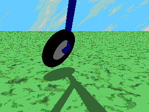
US6976687B2. Prior: 1999 US09434371 Active, 2000 US09708028 Active, 2002 US10331558 Active, 2004-06-25 US10876497 Expired - Fee Related, 2004-11-18 US20040227318A1 Application, 2005-12-20 US6976687B2 Grant.

Control Theory in Robotics

[RoboTrikke] Sachin Chitta, Peng Cheng, E. Frazzoli, V. Kumar. "RoboTrikke: A Novel Undulatory Locomotion System". In Proc. IEEE Int. Conf. Robotics and Automation, pages 1597-1602, Barcelona, Spain, April 2005. DOI: 10.1109/ROBOT.2005.1570342.

[Roller-Walker] Gen Endo and Shigeo Hirose. "Study on Roller-Walker: Multimode steering control and self-contained locomotion". In Proc. IEEE Int. Conf. Robotics and Automation, pages 2808-2814, San Francisco, April 2000. DOI: 10.1109/ROBOT.2000.846453

Papers

[CarveABike] Sachin Chitta, V. Kumar. "Biking Without Pedaling". November 2006. Chitta, Sachin. “Biking Without Pedaling.” (2006).

[Air Force] Charles E. Clauser, et al., Air Force Systems Command, Wright-Patterson Air Force Base, Ohio. August 1969. Pub AD-710 622.

[Moment Of Inertia] Dr. J. B. Tatum. Chapter 2, 'Moment Of Inertia', section 2.8. University of Victoria. 2017. http://astrowww.phys.uvic.ca/~tatum/classmechs/class2.pdf, 2019.

[physics] Michael Lastufka, "Body-Powered Trikke Physics" June 2020.

[calibrated] Michael Lastufka, "Empirical 2nd Degree Friction Model Solution" June 2020.

[behaviors] Michael Lastufka, "Survey of Simulated Trikke Behaviors" June 2020.

[magic] Michael Lastufka, "Trikke Magic: Leveraging the Invisible" June 2020.

Other

[George Box] Box, George E. P. (1976), "Science and Statistics" (PDF), Journal of the American Statistical Association, 71: 791–799, DOI: 10.1080/01621459.1976.10480949.

[Nonstandard Analysis] MathWorld: Nonstandard Analysishttp://mathworld.wolfram.com/NonstandardAnalysis.html. 2019.

[POV-Ray]http://www.povray.org/, 2019.

[sportsdefinitions.com] SportsDefinitions.com. http://www.sportsdefinitions.com/, 2019.

[EzyRoller] EzyRoller LLC. 22588 Scenic Loop Rd., San Antonio TX 78255 - USA. https://www.ezyroller.com/, 2019. Email: info@ezyroller.com

[Flicker] Yvolution USA Inc. 2200 Amapola Court, Suite: 201, Torrance, CA 90501 – USA. https://yvolution.com/, 2019. Email: support@yvolution.com

[PlasmaCar] PlaSmart Inc. 228-30 Colonnade Road, Nepean, Ontario K2E 7J6 - Canada. https://plasmarttoys.com/, 2019. Customer Service 1-877-289-0730 Ext. 214

[Citizen Science] SciStarter. https://scistarter.com/citizenscience.html, What is citizen science?, 2019. Email: info@scistarter.com