Empirical 2nd Degree Friction Model Solution

Draft: 2 June 2020

Validation of kinematic and dynamic computer models require calibration of various components. A friction model is fundamental to many, especially nonholonomic systems like Trikke locomotion. This work demonstrates a method to find reasonable coefficients for a 2nd degree friction model of a vehicle; a Trikke T78 Air. The author starts with the general equations for a friction and coasting model derived from basic principles. In the field, a data collection procedure provides empirical coasting data from two directions to aid in the elimination of slope and wind effects. The models are coded for iteration in a Monte Carlo algorithm to estimate the friction coefficients. Ideal models for each direction and the combined data are compared to the data and incorporated into the target Trikke Model for evaluation. The Trikke Model simulation is presented in a separate work.

A Reasonable Friction Model

Trikkes have fascinated me by their graceful sweeps, turns and athletics ever since viewing the first infomercial on TV in the early 2000s. As a hobby, I have spent many hours experiencing, pondering and modeling the dynamic interactions between the rider and Trikke kinematics. This activity included deriving its [physics], modeling via [simulation] trying to understand its [behaviors] and improving [riding] techniques. Fundamental to the models is a friction model. Without it, conclusions can barely claim to show any qualitative results, let alone quantitative.

Rough Dimensions of a Trikke

Trikke locomotion has three possible energy inputs; "jetting", "carving" and "castering". Jetting simply leverages the rider's intentional rotation about the Trikke's turn-center into movement of the Trikke-Rider System's (TRS) center of mass along its orbital path. This momentum transfer is proportional to the ratio of the turn-radius of the center of mass to that of the turn-radius of the path. This is the most fundamental energy input mechanism; carving and castering both feed into it.

Carving converts the rider's linear and angular body impulses into motion along the front wheel path. Jetting is the rotational component of carving. Its linear component is Direct-Push and Pull. Ground friction constrains both to align with the guide-wheel path. Forward motion due to carving greatly exceeds that due to castering, but the nuances of both techniques are fundamental to meeting all the challenges that riding a Trikke encounters.

Castering releases momentum along the front wheel path as a turn completes. The geometry of the wheel mount and yoke articulations synergistically pull the rider on the trailing frame into the turn and then push the trailer further into the turn, as the guide-wheel passes the forward direction. As the turn completes, the trailer rotation is transfered as a jet through the guide-wheel contact point. The additional force of rotating the trialer is passed to the rider in turning the handlebars, but is ameliorated by the large mechanical advantage of the steering column in cambering.

Obtaining ratios between the effects of these mechanisms relies heavily on the friction model. For example, too much friction at low speed squelches castering related motion. Too little friction and caster-push dominates unreasonably. Part of this paper's length is due to deriving the equations and models from first principles. This process of fitting coasting data applies to many vehicular modeling calibrations of similar nature.

This paper is organized as follows:

A General 2nd Degree Friction Model
A General Coasting Model
Effects of Slope and Wind on Models
Data Collection Procedure
The Data
Monte Carlo Parameter Estimation
Friction Coefficient Solutions
Combined Data Models
Combined Ideal Friction Model
Results Evaluated Against the Data
Results Evaluated Against the Trikke Model
Conclusion
Glossary
Appendix A: Data
Table A.1 Coasting from East
Table A.2 Coasting from West
Table A.3 Ideal West Coast Model
Table A.4 Ideal East Coast Model
Table A.5 Combined Coast Model
Table A.6 Theory vs. Average Polynomial
Table A.7 Simulation vs. Theory
Appendix B: Derivations
Derivation of Coasting Model Velocity via Time and Acceleration
Derivation of Coasting Model Time via Velocity
Derivation of Coasting Model Velocity via Time
Derivation of Coasting Model Distance via Time
Derivation of Terminal Velocity
Derivation of Effect of Slope on Friction Coefficients
Derivation of Effect of Wind on Friction Coefficients
Coefficients and Combined Effects
Appendix C: Algorithms
Monte Carlo Parameter Estimation
Iterative Coasting Simulation
Iterative Terminal Velocity Simulation
References

A General 2nd Degree Friction Model

In college physics classes, we learn several simple ways to model friction. The various factors at the interface exposed to friction are typically:

the nature of contact at the interface: dry, sticky, wet, bumpy, spiked, etc.
the load on the interface
the relative speed of the surfaces at the interface
the thermal properties of the interface
the mechanical properties of the interface

Each has a few physical parameterizations, considerations and disclaimers. Friction is just plain difficult to characterize and even harder to quantify consistently.

Taking an empirical approach, friction is modeled as a curve fit to data. Starting from basic principles, a reasonable and simple friction model for just about any wheeled vehicle can be found.

Generally, friction is modeled as:

F = -μ Λ

where F is the friction force in Newtons; μ is a scalar (unit-less) friction coefficient; and Λ is the load on the interface in Newtons.

Often, μ is a function of the velocity at the interface. For dry interfaces, μ might be modeled as a constant a. With bearings, the model may include a direct velocity component multiplied by a coefficient b. Wind and other fluids operating on the interface often introduce a v² dependence scaled via a coefficient c.

μ = a + b v + c v²

μ - Scalar friction model general coefficient. Often refined as a function of other processes that affect it over time.
a - Scalar friction model coefficient representing dry, non-deforming rubbing actions.
b - Friction model coefficient in s/m representing deforming actions.
c - Friction model coefficient representing viscous actions in s²/m.
v - Instantaneous velocity in m/s.

This is the form of the friction model used in this field study attempting to match the values of the coefficients a, b, and c with the measured kinematic data.

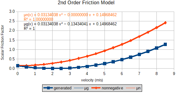
Figure 1: 2nd-Degree Polynomial Friction Model

Figure 1 illustrates a 2nd-degree polynomial friction model for μ(a,b,c) with coefficients set to the values computed in this study (blue curve). Note, the coefficient a is the y-axis intercept. Coefficient b turned out to be negative, pulling the low velocity end of the curve down toward 0; almost no friction at all. The orange curve and equation demonstrate what happens to the friction when coefficient b is zero. More force is required to attain a specific speed, even at low speed. The velocity-squared coefficient, c, is the one that eventually limits the speed of the vehicle to its terminal velocity by greatly increasing friction as speed climbs.

To find the "abc"s of this friction model, a kinematic model containing it was developed for coasting and a stochastic parameter estimator employed. Maximum or terminal velocity is also examined, as the model must fit that quality as well.

A General Coasting Model

Coasting is the simplest motion of a Trikke. It does not rely on the rider's skill or strength, perhaps only balance. Under ideal experimental conditions, friction alone brings the Trikke to a stop. For a given initial speed, v₀, it coasts a distance, d_c, in a certain time, t_c. Given enough trials, the data {v₀, t_c, d_c} can be used to solve for the friction model coefficients a, b and c.

Start with one of the more intuitive ways to model the kinematics of coasting, the sources of force on the Trikke to obtain an "equation of motion". The simple friction model above equates to a force known as drag. The total force and only force on the Trikke is drag. Each term in the friction model represents a different drag source, but the combined effect is "felt" by the whole system via mass times acceleration M Ɑ, the total system force.

Equation of motion for coasting (EOM_c)

M Ɑ(v(t)) = L g (a + b v(t) + c v(t)²)

M - Total Trikke and Rider mass in kg.
Ɑ - Instantaneous acceleration in m/s².
v - Instantaneous velocity in m/s.
t - Instantaneous time in s.
L - Load on the Trikke bearings in kg. Same as M less the axle and the wheel mass.
g - Gravitational acceleration at sea level in m/s². g = -9.8107 m/s²
a - Scalar friction model coefficient representing dry, non-deforming rubbing actions.
b - Friction model coefficient in s/m representing deforming actions.
c - Friction model coefficient representing viscous actions in s²/m.

Only the decelerating force of friction acts on the mass, M, at time, t, via the instantaneous acceleration;

Ɑ(v(t)) = L g (a + b v(t) + c v(t)²)/M

At v = 0 m/s, the Trikke has rolled to a stop over the coasting distance, d_c in time, t_c. Deceleration is not zero, but is equal to (L g a)/M. Coefficient a must be positive for the Trikke to stop since g is negative.

Note: any instantaneous value of v becomes the initial value, v₀, for coasting the rest of the distance.

From the EOM_c, a cascade of equations for kinematic variables can be derived. The above acceleration equation is solved algebraically for instantaneous v(t) using the "quadratic equation". Next, separate the terms in v from those in t and integrate via the differentials ∂v and ∂t respectively to get the coasting time in terms of velocity, t(v). The solution includes the arctangent function introducing a periodic nature to the model. Inverting the arctangent allows solving algebraically for v(t). Integrating by the time differential, ∂t, gives coasting distance in terms of time, d(t). The results are enumerated in Table 1, and the derivations carried out in Appendix B.

Terminal Velocity

On the other end of the kinematic landscape, the speed of a Trikke is self-limiting. As speed increases, wind resistance increases most noticeably, until nearly all the force, R, the rider inputs to the system goes into moving air out of the way. There may also be some tire deformation and heat to overcome as the force exerted on the tread by pebbles is proportional to the wheel speed. On a smooth surface, the main decelerant is air. The maximum speed achievable at a given input of R is called "terminal velocity". For a Trikke with a good, strong rider, terminal velocity on flat ground with no wind may be 12 mph (5.36448 m/s).

The equation of motion for this situation EOM_{v_t} includes Not only the force of friction, but also the rider's force, R, in Newtons. Unlike direct force application through bicycle pedals and gears, this R-force is administered indirectly through other momentum transfer mechanisms. Never-the-less, this simple form of EOM_{v_t} is the same for both vehicles and many others.

M Ɑ(t) = R + L g (a + b v(t) + c v(t)²)

M - Total Trikke and Rider mass in kg.
Ɑ - Instantaneous acceleration in m/s².
t - Instantaneous time in s.
R - Trikke Rider's effort to maintain a constant forward force each carving cycle in Newtons.
L - Load on the Trikke bearings in kg. Same as M less the axle and the wheel mass.
g - Gravitational acceleration at sea level in m/s². g = -9.8107 m/s²
v - Instantaneous velocity in m/s.
a - Scalar friction model coefficient representing dry, non-deforming rubbing actions.
b - Friction model coefficient in s/m representing deforming actions.
c - Friction model coefficient representing viscous actions in s²/m.

Assume the rider drives the Trikke forward with a constant force during a duty cycle. Terminal velocity peaks when R equals drag so that M Ɑ(t_t) is 0. t_t is the "terminal time" taken to coast to a stop from an initial velocity. The Trikke friction model must be able to express a terminal velocity near 5 m/s at an achievable value for R. Starting with the equation of motion for terminal velocity, another cascade of kinematic variables can be solved. These expressions are similar to those for coasting, but signs on some terms are swapped and inverse hyperbolic tangents appear.

Unfortunately, some of them are very sensitive to small changes in the variables and lead to unwieldy values that are highly periodic and difficult to interpret. Instead, a simple iterative algorithm was developed to produce the desired data to confirm model compliance. The better behaved equations related to achieving terminal velocity are derived in Appendix B.5 and presented in Table 1.

Table 1: Coasting Model Derived Equations
Description	Equation Derived from EOM1 and 2
Equation of Motion for Coasting	M Ɑ(v(t)) = L g (a + b v(t) + c v(t)²)
Velocity via Time and Acceleration	v(Ɑ,t) = -b/(2 c) + \[b² + 4 c (a - M Ɑ(t)/(L g))]/(2 c)
Coasting Time via Initial Velocity	t_c = 2 M (tan^-1(b/\[u]) - tan^-1((2 c v₀ + b)/\[u]))/(L g \[u]), u = 4 a c - b²
Initial Velocity via Coasting Time	v₀(t_c) = ((b - \[u] tan(G(t_c)))/(1 + b tan(G(t_c))/\[u]) - b)/(2 c), G = L g \[u] t_c/(2 M)
Coasting Distance via Coasting Time	d_c = M (log(((b sin(L g \[u] t_c/(2 M)) + \[u] cos(L g \[u] t_c/(2 M)))²)/\[u]²) - b L g t_c/M)/(2 c L g)
Equation of Motion for Terminal Velocity	M Ɑ(t) = R + L g (a + b v(t) + c v(t)²)
Terminal Velocity via Rider's Effort, R	v_t(R) = -b/(2 c) +/- \[b2 - 4 c (a + R/(L g))]/(2 c)
Rider's Effort via Terminal Velocity	R(v_t) = -L g (a + b v(t) + c v(t)²)

Effects of Slope and Wind on Models

Beyond the models considered so far, there are at least two factors that need to be addressed in actual data: slope and wind. Under perfect laboratory conditions, the coasting runs would be executed on a perfectly flat surface in an enclosure that stifles any wind or draft; perhaps inside a warehouse or airplane hangar. Part of this exercise was to see if the effects of slope and wind could be accounted for and eliminated from the final model.

It seemed reasonable that this could be done by taking pairs of measurements from opposite directions, east and west in this case. Teasing the mathematical representation of slope and wind resistance from the theory using the abc friction coefficients for the east and west data was pretty straight-forward. The results are presented in Table 2.

Table 2: Coefficient Perturbations due to Slope and Wind
Description	Equation	Comments
Effect of Slope	a' = a + sinθ M/L	Up: θ > 0 a increases Down: θ < 0 a decreases
Effect of Wind	a' = a + σ k ρ A w²/(2 L g)	With: w, σ > 0 b decreases Into: w, σ < 0 b increases
Combined Effects	a' = a + sinθ M/L + σ k ρ A w²/(2 L g)	See above effects
a derived from a'	a = (a'₁ + a'₂)/2	a'₁ and a'₂ from data sets measured coasting in opposite directions.

a' - Treated like the friction model scalar coefficient a, it includes the contribution of the rider's input force.
a - Scalar friction model coefficient representing dry, non-deforming rubbing actions.
θ - Angle of pavement slope in radians. θ < 0 is down hill. θ = 0 is level ground. θ > 0 is up hill.
M - Total Trikke and Rider mass in kg.
L - Load on the Trikke bearings in kg. Same as M less the axle and the wheel mass.
g - Gravitational acceleration at sea level in m/s². g = -9.8107 m/s²
σ(w) - Signum function. Returns the value 1 with the same sign as w.
k - Aerodynamic scalar form factor. Typical values are between 1.3 for a flat wind-facing surface and 0.3 for a 3-ogave nose cone.
ρ - Dry air density at sea level under standard temperature and pressure. 1.225 kg/m³
A - Forward cross-section area presented to the fluid flow. Units are m².
w - Constant wind speed in m/s². Wind traveling with the Trikke is positive. Against the Trikke is negative.

Table 2 sports some new variables. a has a slope and wind confounded counterpart a'. a' can be solved numerically from the measured data. But it "confounds" the effects from slope and wind with the flat, no-wind value a as indicated in Table 2. Without wind and slope, a best expresses wheel/axle related friction. As the slope and wind forces have no vehicular velocity dependence, their effects do not perturb friction model coefficients b or c. The values to solve for from the Trikke coasting model are the no-slope, no-wind coefficients a, b, and c, but a' must be found first.

Unfortunately, Even once the friction coefficients for the opposite coasting runs are known, the above equations cannot be solved for the slope angle, θ, or the wind speed, w, since they are both confounded in a'. The best that can be done is find a = the average of the a's from opposite directions.

Data Collection Procedure

A single Trikke T78 Air, driven by the author provided measurements using a sports tracking watch and uniform paving slabs, each 15-feet across, in the parking lot of a huge warehouse. Being 6-tenths of a mile around and at least three-stories tall the warehouse provides the best wind block and flattest terrain in the area.

A few days of practice trials preceded the final collection of data. Even though the wind was mostly out of the South, there was a noticeable difference in measurements from the east vs. those from the west. It is likely that the visually flat parking lot is tilted down toward the west.

On November 8, 2018, 20 measurements of v₀, t_c, and d_c were collected and on the 21^st another 24 measurements were made under similar environmental conditions. Runs ranged from faster initial speed reducing to slower. An attempt was made to run initial speeds in pairs, first from the west then from the east. In this way, it was hoped 10 or 12 pairs at different initial speeds would cover the typical Trikke speed range. A 5 mph breeze out of ENE evidently turned to run parallel to the long aspect of the building, but affected measurements much more than the stronger winds from the South experienced in preliminary trials.

Data Collection Procedure:

Carve the Trikke up to an estimated initial speed judging by experience from the east or west close to the warehouse docking stations. Begin coasting.
Click the timer lap button on the sports tracking watch upon crossing a designated line perpendicular to the coasting path between two pavement slabs. Later, read this initial speed from the tracker data at this "lap" on the website associated with the sports watch. Note that it is difficult to accelerate a Trikke with only one hand on the handle bar and the other clicking the watch. However, it does not affect coasting.
Increment a mental count upon crossing each subsequent line between paving slabs. Each 15-foot slab gives plenty of time to notice the septa between them.
Click the lap button again when the Trikke stops, obtaining the time for the coasting run. Note any partial block covered to one-tenth of a slab length, which is easy to estimate.
Record the the run number, path direction (East or West), slab count, and partial coverage.
Upon completion, access the sports watch website to upload the tracking data results; initial velocity, v₀, and coasting time (called moving time), t_c, for each "lap". Copy each lap's data to a spreadsheet. For each coasting run (lap), the path, p_c (from west or east), and the coasting distance, d_c, are taken from the trial field records in terms of slabs traversed.
Each run record includes (p_c, v₀, t_c, d_c).

The Data

Data collection resulted in two sets when grouped by p_c, of multiple data points {v₀, t_c, d_c}. Figure 2 and Figure 3 presents the data collected according to the above procedure. See Appendix A Tables A.1 and A.2 for the numbers. To mitigate slope and wind factors, data was collected alternating runs east-to-west and west-to-east across the leeward side of the building, protecting from south winds. Unfortunately, on Nov 8, 2018 the wind was out of the ENE at 5 mph according to the sports tracking data website and 5 mph from the North on Nov 21, 2018. Both breezes seemed to align along the east-west axis of the building. As can be seen in the plots, there is much overlap in the data.

By plotting the coasting distance against the coasting time, the data was expected to fall close to a 2nd-degree polynomial curve based on plotting simulated coasting results and the form of the derived equation d(t). The initial speed for each data point was expected to form a monotonic increasing sequence of labels on the curve. With rather wide variation, the data tended toward this expectation. However, the resulting curves show two very different populations. The data starting from the east side of the lot measures almost twice the distance and 1.5 the time range for coasting to a stop than the data coasting from the west side.

Much "noise" in the data led to pruning the points that fell farthest from the 2-degree polynomial trend lines. Coasting distance measured within 23 cm of error. Coasting time was taken from the "moving time" in whole seconds from the sports watch website lap data. The lap interval time from the website is often too long - the watch reports time every few seconds regardless of the actual lap-click time according to sports watch forum.

Figure 2

Figure 2 shows coasting distance, D_c, plotted against coasting time, T_c, with initial speed, v₀, labeling each measurement. Coasting proceeded from east to west along the leeward side of the building. Different colors designate points from both trial days. Those from the second day in red, seem more scattered at the lower end of the trend line. Removing outlying points (X) farthest from the developing 2nd degree polynomial made it curve up more. This did not straighten out the v₀ sequence. It is rather noisy data.

Figure 3

Like the data obtained by coasting from the east side of the parking lot, the data from the west side shows out-of sequence v₀ and much more scattering. Removing the outlying measurements farthest from the developing trend line turned it from a frown to slightly happier than a line; 9 points removed out of 22! Again the v₀ labels tend to increase, but many regress.

These two sets of rather wild data were "smoothed" by filtering the data that was most divergent from curve-fitting to produce a reasonable 2nd-degree polynomial trend line. A nice progression of v₀ did not appear on this line, but with a few well chosen data points an "ideal" model of the data, certainly not unique, was achieved.

To construct an ideal model of the two data sets, solve for the friction model "abc"s of both curves using 5 selected data points from each set. This required a point selection process and selection of a solver. Using these coefficients, an ideal "back-model" can be constructed by evaluating either the d(t) and v(t) model equations or by an iterative coasting simulation based on the Coasting Equation of Motion. This gives insight into the distribution of the initial speeds on the curves as well. With the back-models, it is possible to obtain the average of their trend line polynomials to get a combined back-model closer to representing flat, calm coasting run data.

Solving for a, b, and c analytically is likely not possible or feasible. Instead, the author developed a simple Monte Carlo Parameter Estimator requiring a seed, a finite number of data points and a least sum of squares evaluator to do the job. But which n points should be selected?

Monte Carlo Parameter Estimation

The author created a simple Monte Carlo Parameter Estimation (MCPE) method, sketched in Appendix C, that requires evaluation of the initial velocity, v₀, and coasting distance, d(t), derived equations, with inputs (t_c, a, b, c) to obtain outputs (v₀, d_c). It uses a set of randomly generated triples (a, b, c) from seeds and an evaluation function that compares simulation outputs with the measurement d_c for a set of 5 t_cs. It is an iterative process that stops when the evaluation reaches 2100 iterations, a large but arbitrary number that took a few minutes to process.

The initial set of seeds were estimated by "playing" with a simulation. 0.01 was found adequate for each parameter a, b, and c. A random value in the range (-(10^-i)/2, 10^-i/2) is added to each coefficient of a seed triple to generate the next set of triples for evaluation. The i cycles through the range [3,6] tweaked these digits to produce good variation. Not all seeds produce valid coasting trials. If a set of a, b, c values caused an error during evaluation, the trial was terminated with coasting distance set to 0 and continued with the next seed.

Friction Coefficient Solutions

The MCPE described above determined solutions for the friction coefficients a, b, and c for both east and west data. While the trend lines of the data were useful for selecting key data points for this step, the trend lines themselves were not used. Running the MCPE many times seeded by the lowest scoring "abc"s, converged on the friction model coefficients documented below.

Coasting from the East

Points used to solve for the friction coefficients were close to the trend line and monotonic in initial velocity, v₀. "Abc"s from the MCPE solution were used to generate an Ideal model. Table 3 shows the key measurements used to solve for a, b, and c with the post-solution deltas of the key points. The least-squares score of the ΔD_cs are also shown; they sum to the score in the paragraph below.

Table 3: Key East Coast Measurements and Model Deltas
v₀ (m/s)	Ideal Δv₀ (m/s)	T_c (s)	D_c (m)	Ideal ΔD_c (m)	Score
1.83	-0.03	7	12.802	-4.923279	24.238674
1.97	0.33	11	16.916	-0.882538	0.778873
2.41	0.69	19	34.290	3.144353	9.886955
3.89	2.9	27	72.238	-0.723161	0.522962
4.65	N/A	31	89.154	-0.147817	0.021850

The MCPE algorithm achieved a total least-squares deviation score of 35.44931301 after many runs, refreshing the seed with the best estimates, until no lower scores were produced. The set of coefficients with the lowest total least-squares deviation score follows. The Ideal coasting model using the estimated 2nd-degree polynomial friction model coefficients a, b, c is shown in Figure 4.

a = 0.06118032, b = -0.04212474, c = 0.00875603

To compare the measured data to ideal data calculated using the above coefficients, a range of coasting time from 0 to 30 seconds was input into the derived equations for coasting distance and velocity. See the numbers in Table A.4.

Figure 4: Ideal Coasting Profile from East-Side Data

Note that the initial velocities increase rapidly near the 30 second mark. Also, the last one in the graph is -30.90 m/s. There is a pole (infinity) between the 21.00 and the -30.90 values, indicting that the v(t) equation changed foliations due to the tangents cycling. To see this from a different perspective, d_c and t_c were plotted against v₀ in Figure 5.

Figure 5: Ideal Coasting Distance and Time VS. Initial Velocity from East-Side Data

These are logistic curves showing that higher initial coasting velocities result in vanishing distance gains. Initial velocity values were cut off at 10 m/s since plotting the next v₀, 21 m/s, would double the length of the plot needlessly.

Coasting from the West

Key data points used to solve for the friction coefficients for coasting from the west are shown in Table 4 with their post-solution deltas and scores.

Table 4: Key West Coast Measurements and Model Deltas
v₀ (m/s)	Ideal Δv₀ (s)	T_c (s)	D_c (m)	Ideal ΔD_c (m)	Score
1.61	0.49	8	11.887	1.13083	1.278777
2.46	0.84	10	17.831	0.147302	0.021698
2.77	N/A	16	27.432	-0.248329	0.061667
3.62	N/A	20	35.433	-0.300322	0.090193
4.16	N/A	22	44.577	-0.001985	0.000004

The MCPE algorithm achieved a total least-squares deviation score of 1.45233962 after many runs, refreshing the seed with the best estimates, until no lower scores were produced. The set of coefficients with the lowest total least-squares deviation score follows. The Ideal coasting model using the estimated 2nd-degree polynomial friction model coefficients a, b, c is shown in Figure 6.

a = 0.33573268, b = -0.35944849, c = 0.09874126

Figure 6: Ideal Coasting Profile from West-Side Data

In this data set, the initial velocities increase rapidly near the 11 second mark and the periodic nature of the model appears in three foliations. Two poles are easily identifiable. d_c and t_c are plotted against v₀ in Figure 7 where the foliations stand out.

Figure 7: Ideal Coasting Distance and Time VS. Initial Velocity from West-Side Data

These are 3 sets of logistic curves each showing that higher initial coasting velocities result in vanishing distance gains. Only the bottom foliation is physically coherent making this model limited in use.

Combined Data Models

Plotting the two data sets on the same chart with their 2nd-degree polynomial trend lines produced Figure 8 below. Blue symbols pinpoint the filtered east coast data with its trend line equation at the top; red symbols locate the filtered data from the west. Its equation is in the middle. Note they intersect at a coasting time of about 14 seconds.

The third trend line, in purple, is also a 2nd-degree polynomial. The coefficients of the two filtered data sets were averaged to produce the combined "Dc(Tc)avg" curve. Initial velocities were computed along the curve after solving the friction coefficients and applying v₀(t_c). Note another foliation begins around 23 seconds with a negative initial velocity; the corresponding coasting distances and times are not realizable starting at those speeds.

Figure 8: Averaged Trend Lines with Initial Velocities

Combined Ideal Friction Model

Coasting distance points selected from the averaged curve with evenly spaced coasting times of 8, 12, 16, 20 and 24 seconds primed the MCPE algorithm to solve for the friction coefficients. See Appendix A Table A.5 and A.6 in columns 4 to 6 for the numbers. The v₀ at the 24 time mark does not have a valid interpretation in the model. However, its corresponding coasting distance and time pair is still a good extreme end point for estimating the friction coefficients. Table 5 shows the key points selected from the combined model curve used to solve for a, b, and c with their post-solution deltas. The least-squares score of the ΔDs are also shown; they sum to the score in the paragraph below.

Table 5: Key Combined Coast Measurements and Model Deltas
v₀ (m/s)	T_c (s)	D_c (m)	Ideal ΔD_c (m)	Score
1.99	8	12.024	-0.124	0.015376
2.21	12	20.154	0.15	0.0225
2.48	16	29.697	-0.046	0.002116
3.19	20	40.653	-0.003	0.000009
-1.34	24	53.020	-0.001	0.000001

The MCPE algorithm achieved a total least-squares deviation score of 0.04016694 after many runs, refreshing the seed with the best estimates, until no lower scores were produced. The set of coefficients with the lowest total least-squares deviation score follows. Because the deviation score is so low, the Ideal coasting model using the estimated 2nd-degree polynomial friction model coefficients a, b, c is essentially the purple average curve shown in Figure 8.

a = 0.14968462, b = -0.13434041, c = 0.03134038

Coasting distance and time as a function of initial velocity is shown in Figure 9. The v₀ range represents typical Trikke operating speeds on flat ground. The gain in coasting distance from an initial velocity of 3.74 m/s to 5.33 m/s is only 4.361 meters and one second of coasting time. In reverse, this represents well the experientially measured terminal velocity condition as the c v² self-induced wind speed term dominates.

Figure 9: Ideal Coast Distance and Time Logistic Curves

Results Evaluated Against the Data

These are the conditions the friction model must satisfy to be considered a realistic, validated model.

Points on the combined coasting curve averaged polynomial trend line in Figure 8
1. ought to be close to those in Table A.6 generated using the combined ideal friction model coefficients and derived model equations.
2. They should also be a close fit to the iterative simulation which is implemented in the Trikke dynamics simulation, Table A.7.
According to the analysis, the friction model coefficients b and c ought to closely match those determined for both measured data sets. See Table 6.
Coefficient a in the combined ideal coasting model should be the average of those determined for each measured data set. See Table 6.
Furthermore, when calculating the combined ideal friction model in a terminal velocity simulation, speed ought to top out around 5.3 m/s at the high end of the rider's force range as in Figure 10.

Examine the evidence more closely.

1.a) d_c calculated via the averaged polynomial equation in the range 0 < t_c < 30 at intervals of one second, compared favorably with theory in the same range. A sample standard deviation of just under half a meter resulted using the Coasting Distance via Coasting Time equation, and no time deviation with the Initial Velocity via Coasting Time equation recorded in Table A.6.

1.b) The iterative coasting simulation requires a starting velocity, so it cannot be directly compared to the averaged polynomial equation. Rather, the theory that was compared to the averaged polynomial curve in 1.a, was compared with the simulation, both producing t_c and d_c. Using a range of 0 < v₀ < 12 m/s incremented by 0.5 m/s was more than adequate. Theoretical values of t_c, Coasting Time via Initial Velocity, d_c via the Coasting Distance via Coasting Time equation, and v₀ (again) via the Initial Velocity via Coasting Time equation achieved sample standard deviations of zero seconds, little over 1.5 millimeters, and zero meters per second (only one was off by 0.01 m/s) respectively in Table A.7.

2) Table 6 shows the difference in coefficients from the three friction models; east, west, and combined (both). Coefficients b and c are very different among the three sets. Even though the curve coefficients were averaged to get the curves the models support, there are no obvious reasons to expect that the combined coefficients would lay between those of the other models. Nicely they do. However, differences in the friction models of this size affect the coasting and terminal velocity models significantly. Perhaps there are other significant friction processes affecting coefficient b and c.

Table 6: Ideal Friction Model Coefficients and Deltas
Data	a	Δa	b	Δb	c	Δc
East	0.06118032	0.0885043	-0.04212474	-0.09221567	0.00875603	0.02258435
Both	0.14968462	0	-0.13434041	0	0.03134038	0
West	0.33573268	-0.18604806	-0.35944849	0.22510808	0.09874126	-0.06740088

Table 6 also shows the differences in coefficient a for each friction model. The average for the east and west models is,

a = (a_e + a_w)/2 = (0.06118032+0.33573268)/2 = 0.1984565

which is 32.6% higher than the 0.14968462 value for the combined friction model. Further experimentation with the selected input keys used in the MCPE algorithm may yield a measure of the sensitivity of the MCPE algorithm and indicate whether this amount of skewness is meaningful. It seems it must be based on sensitivities in the Trikke simulation which are beyond the scope of this paper.

4) The iterative terminal velocity simulation shows a range of rider input force that likely runs much higher than typically achievable. Note, the terminal velocities skirt the 5 m/s line fairly early in Figure 10 indicating that a rider will encounter difficulty achieving higher speeds. According to the combined friction model the lowest force able to initiate motion is about 115 N. A rider's input force must start at this value. This force seems unrealistically high for a 70 kg rider and the ease with which a Trikke will roll, but the difficulty of rising above 5 m/s does not seem out of order. However, the Trikke simulation shows initial forward impulses due to direct-push alone can easily reach 100 N-seconds.

Figure 10: Simulated Speed Limit Around 5 m/s

Results Evaluated Against the Trikke Model

The iterative coasting simulation uses an initial velocity and the friction model to determine the coasting distance and time. The Trikke simulation is much more complex, but subsumes this algorithm, matching its results very closely when the friction model determined in this study is used. The Trikke simulation is based on conservation of momentum, i.e., velocity, rather than force, though impulse is important.

Achieving terminal velocity in the Trikke simulation is very different from the iterative terminal velocity simulation. User inputs are modeled in a cyclic manner with changing impulse and momentum rather than as a continuous average force. So the times and distances needed to achieve terminal speeds are probably much lower in the simple algorithm. However, the terminal velocity itself shows similar outcomes.

The friction model affects the Trikke simulation in a few other ways that can provide a sense for the validity of the friction model.

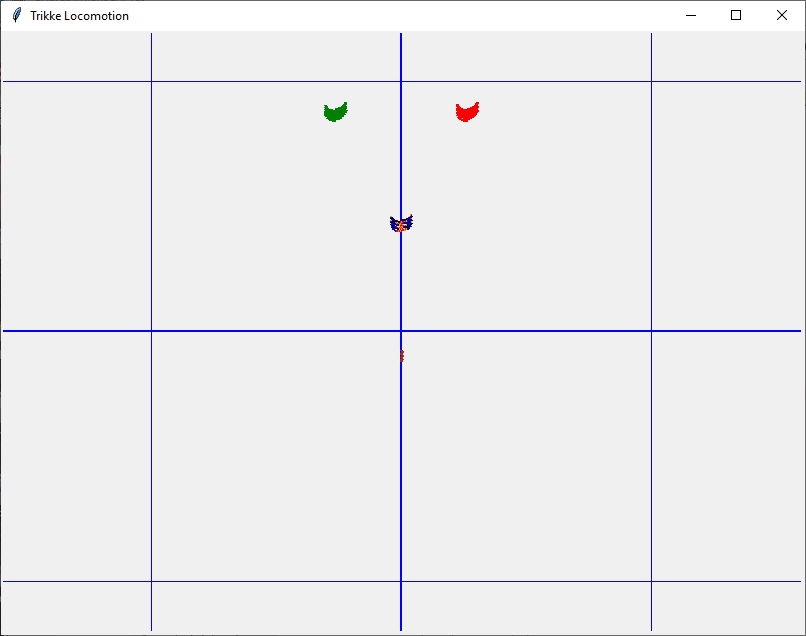
A Trikke does not start from a stop easily when the rider employs only caster with feet planted on the arm-decks. Caster is created when a Trikke's offset front wheel is turned quickly. The articulation of the steering column and the frame shifts forcefully to one side creating an impulse that pulls the frame into the turn. The rider and trailing frame gain angular momentum producing a weak jet rotation. As the rider continues to steer through 0-degrees in the same direction, the articulations release the jet rotation along its path. Turning the drive wheel passes the jet-creating force to the rider's upper body. Castering slightly increases the momentum and thus the speed of the whole system.
There may be some "crawling" when executed correctly, but generally little ground is gained. Riders must concentrate to be sure they are only using caster. The following image was produced under typical "caster only" conditions for eight cycles. Brown marks the drive-wheel path. The blue traces the rider's center of mass, while orange indicates reverse motion. Green indicates the right wheel path; the left is red. The blue squares are one-meter.
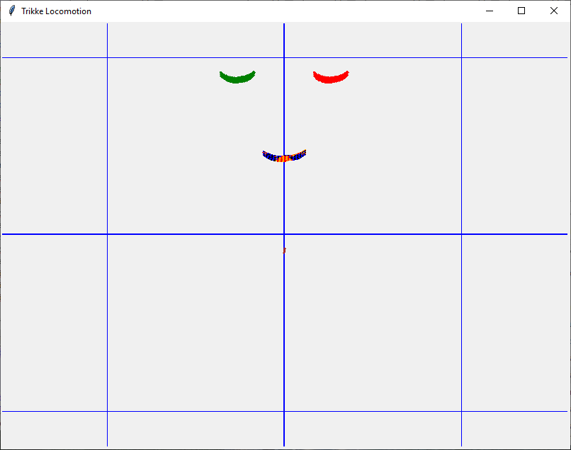
A Trikke starts a bit better when the rider employs caster and camber. It's not pretty as illustrated in this simulated scenario of four cycles. Restraining from adding other impulses into the motion is quite difficult for riders. This motion is more of a side-to-side "crawl".
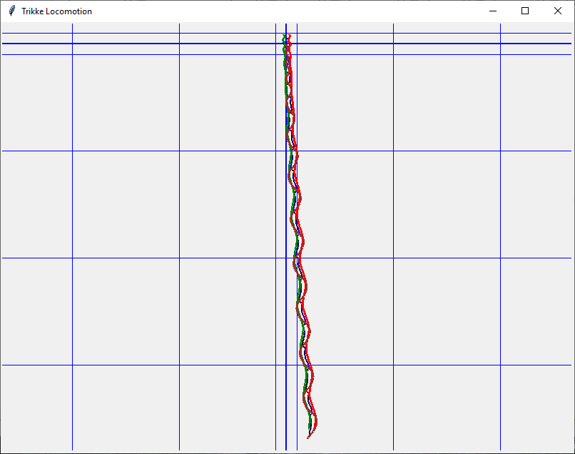
When the rider casters, cambers, and adds forward and/or angular impulses (i.e., carves), the Trikke accelerates gracefully and with less effort once it starts moving. This run illustrates a 3.59 m/s (8.0 mph) per cycle terminal speed along the 44 meter brown drive-wheel path. The small blue squares are one-meter, while the large ones are 10-meters. The rider accomplished 12-cycles in 18-seconds, covering about 37-meters.
Path slope and wind are not included in the Trikke simulation used with this study, but riders become sensitive to these effects and unconsciously compensate their technique.

Conclusion

The analysis in this investigation found the following coefficients of a 2nd-degree polynomial friction equation to adequately represent the performance of the author's Trikke.

μ = 0.14968462 - 0.13434041 v + 0.03134038 v²

Though the experimental measurements were quite noisy and data "pruning" rather extreme, the simulated coasting and independent parameter results (like caster-only propulsion) seem quite reasonable. Typical Trikke simulation acceleration runs matched the experienced, expected terminal velocity expectations. Runs with near-by "abc"s may indicate how sensitive the simulation is to these coefficients. Perhaps other values could work as well and that these results are not so special. On the "con" side, measuring up to the combined data theory didn't fair so well for any of the combined "abc"s.

These conclusions are a bit unfair since the reader has not been properly apprised of the full Trikke simulation. That is the subject of another paper. This one provided a workable friction model that calibrates the Trikke simulation nicely, so its results have some qualitative as well as quantitative credibility. Mission accomplished!

Appendix A: Data

Tables A.1 and A.2

Table A.1	Table A.2

Tables A.1 and A.2 show the data collected from the coasting runs. Runs with the gold v₀ values determined the friction coefficients for each data set. The reddish lines are considered outliers.

Table A.3, A.4 and A.5

Table A.3	Table A.4	Table A.5

West coasting ideal points (T_c, D_c, V₀) calculated from the friction model coefficients highlighted in green and the derived equations for d_c(t_c) and v₀(t_c). Periodicity is quite noticeable in V₀. The first period, up to T_c = 10 seconds, have all three values. Beyond that, the values for V₀ are not relevant. Pairs (T_c, D_c) in the this table's generated data are close to the measured key data points in Table A.1 gold V₀ value rows.	East coasting ideal points (T_c, D_c, V₀) calculated from the friction model coefficients highlighted in green and the derived equations for d_c(t_c) and v₀(t_c). The first period ends just before T_c = 30 seconds, so most points have three relevant values. Pairs (T_c, D_c) in the this table's generated data are not as close to the measured key data points in Table A.2 gold V₀ value rows as those in the West Coast data. V₀ values differ even more.	The ideal curve polynomial coefficients for the coasting data d_c(t_c) calculated using the determined friction model for each measured data set were averaged. Data points calculated from the averaged polynomial coefficients appear in Table A.3. Evenly spaced points (T_c, D_c) with the gold V₀ values from this curve were used to solve for the friction model coefficients highlighted in green. Note a new foliation of the periodic function V₀(T_c) at T_c = 24 seconds.

Table A.6: Theory vs. Average Polynomial

Combined coasting ideal points (T_c, D_c, V₀) calculated from the friction model coefficients highlighted in green and the derived equations for d_c(t_c) and v₀(t_c). The first period ends just before T_c = 24 seconds, so most points have three relevant values. Pairs (D_c, V₀) in generated columns 2 and 3 are nearly and exactly the same as the key data points in columns 4 and 5 gold V₀ rows as those in the Combined Coast data computed using the averaged polynomial trend lines.

Table A.7: Simulation vs. Theory

Starting with the initial velocity range 0 to 12 meters per second , simulated Coasting runs resulting in t_c(v₀) and d_c(v₀) are compared to the Combined coasting ideal data computed from theory and simulated t_c(v₀)s. Coasting distances are off up to 2 millimeters and only one initial velocity is different by a centimeter per second.

Appendix B: Derivations

Derivation of Coasting Model Velocity via Time and Acceleration

The following list of variables appear in the various derivations making up this coasting model. Some of them have different mathematical expressions depending on the context.

Var-Coast: Coasting Model Variables

v₀ - Initial velocity when coasting began in m/s.
d_c - Distance traveled while coasting from the initial velocity to a stop in m.
t_c - Time traveling from v₀ to a stop in s.
t - Instantaneous time in s.
M - Total Trikke and Rider mass in kg.
L - Load on the Trikke bearings in kg. Same as M less the axle and the wheel mass.
Ɑ - Instantaneous acceleration in m/s².
v - Instantaneous velocity in m/s.
g - Gravitational acceleration at sea level in m/s². g = -9.8107 m/s²
a - Scalar friction model coefficient representing dry, non-deforming rubbing actions.
b - Friction model coefficient in s/m representing deforming actions.
c - Friction model coefficient representing viscous actions in s²/m.
u = The scalar binary quadratic form discriminant of the Friction Model in the form of an inverted velocity.
G = A scalar representing something like a load velocity damping-ratio up to time t.

When coasting begins, a vehicle is at initial velocity. While coasting, the vehicle slows down due to friction. Rubbing and rolling of the ball bearings in the wheel hubs, tread grabbing the road, heat transfer with tire deformation, and air resisting movement around the structure produce forces that oppose travel.

At time t = 0, the Trikke is at velocity v₀. When the Trikke coasts to a stop, v = 0 and t = t_c.

The equation of motion for coasting (EOM_c) implements Newton's 2nd Law with the decelerating force of the 2nd-degree friction model.

M Ɑ(v(t)) = L g (a + b v(t) + c v(t)²)

Some of the variables have been parameterized with v and t to emphasize their dependence on time. For most of the derivation, such emphasis is not necessary.

A couple algebraic manipulations sets up a standard polynomial equation in v to solve for v in terms of Ɑ and t.

c v² + b v + a - M Ɑ/(L g) = 0

Choose the + branch since when a = M Ɑ(t)/(L g), the negative branch gives 0, the + gives v > 0

v(Ɑ,t) = -b/(2 c) + \[b² + 4 c (a - M Ɑ(t)/(L g))]/(2 c)

Derivation of Coasting Model Time via Velocity

This derivation uses the coasting model variables.

Start with the equation of motion for coasting. Solve for the acceleration in terms of velocity.

Ɑ(v) = L g (a + b v + c v²)/M

As a sanity check evaluate with some typical values: a = 0.03325321, b = -0.01886216 s/m, c = 0.00481075 s²/m, M = 81.22 kg, L = 79 kg, g = -9.8107 m/s².

Ɑ(v₀=0 m/s) = -0.317320 m/s2

For v₀ = 2.77 m/s, the b coefficient pulls acceleration magnitude down to almost half that at the end of coasting computed above.

Ɑ(v₀=2.77 m/s) = -0.170978 m/s2

Since Ɑ(v) = ∂v/∂t, separate the variables and integrate both sides over their corresponding ranges.

int(∂v/(a + b v + c v²))[v₀,0] = int(L g ∂t/M)[0,t_c]

Look up the solution for the LHS in a reference, the RHS is simple.

Let u = 4 a c - b²

2 tan^-1((2 c v + b)/\[u])/\[u] [v₀,0] = L g t/M [0,t_c]

Evaluate the integration limits.

2 tan^-1(b/\[u])/\[u] - 2 tan^-1((2 c v₀ + b)/\[u])/\[u] = L g t_c/M - 0

Solve for t_c.

t_c = 2 M (tan^-1(b/\[u]) - tan^-1((2 c v₀ + b)/\[u]))/(L g \[u])

Derivation of Coasting Model Velocity via Time

This derivation uses the coasting model variables.

Start with the solution of the coasting time definite integral where the limits are the coasting time, t_c and its corresponding initial velocity, v₀. Solve for the initial velocity in terms of coasting time.

Prepare to open up the arctan with v₀ in it, to isolate v₀.

tan^-1((2 c v₀ + b)/\[u]) = tan^-1(b/\[u]) - L g \[u] t_c/(2 M)

Apply tan() to both sides.

(2 c v₀ + b)/\[u] = tan(tan^-1(b/\[u]) - L g \[u] t_c/(2 M))

Simple algebraic manipulations isolates the velocity on the LHS.

v₀ = (\[u] tan(tan^-1(b/\[u]) - L g \[u] t_c/(2 M)) - b)/(2 c)

Let G = L g \[u] t_c/(2 M), it represents something like the ratio of gravitational acceleration to frictional deceleration.

The general equation for the tangent of a difference combines the tangent expressions.

tan(z-w) = (tan(z) - tan(w))/(1 + tan(z)tan(w))

With z = tan^-1(b/\[u]) and w = G,

tan(tan^-1(b/\[u]) - G) = (b/\[u] - tan(G))/(1 + b tan(G)/\[u])

Now v₀(t_c) becomes,

v₀(t_c) = ((b - \[u] tan(G(t_c)))/(1 + b tan(G(t_c))/\[u]) - b)/(2 c)

Derivation of Coasting Model Distance via Time

This derivation uses the coasting model variables.

Start with the coasting model initial velocity via coasting time equation. Solve for the coasting distance in terms of coasting time, d_c(t_c), noting that v₀(t_c) = ∂d/∂t.

∂d/∂t = ((b - \[u] tan(G))/(1 + b tan(G)/\[u]) - b)/(2 c)

Separate the variables and integrate both sides over their corresponding ranges.

int(∂d)[0,d_c] = int((((b - \[u] tan(G))/(1 + b tan(G)/\[u]) - b) ∂t)/(2 c))[0,t_c]

The integral on the RHS is equal to

M (\[u] log((b sin(G) + \[u] cos(G))²) - 2 b G)/(2 c L g \[u]) [0,t_c]

Evaluate both sides

d_c = M (\[u] log((b sin(G) + \[u] cos(G))²) - \[u] log(\[u]²) - 2 b G)/(2 c L g \[u])

Remembering the difference of logs is the log of their ratio,

log(z) - log(w) = log(z/w)

Apply and simplify by factoring out \[u]. It forms a one with the \[u] in the denominator.

d_c = M (log(((b sin(G) + \[u] cos(G))²)/\[u]²) - 2 b G/\[u])/(2 c L g)

Substitute G back in and simplify.

d_c = M (log(((b sin(L g \[u] t_c/(2 M)) + \[u] cos(L g \[u] t_c/(2 M)))²)/\[u]²) - b L g t_c/M)/(2 c L g)

Derivation of Terminal Velocity

The following list of variables appear in the various derivations making up this terminal velocity model. Some of them have different mathematical expressions depending on the context.

Var-Terminal: Terminal Velocity Model Variables

R - Trikke Rider's effort to maintain a constant forward force each carving cycle in Newtons.
v_t - Terminal velocity in m/s.
d_t - Distance traveled at constant effort needed to speed up to v_t from a stop in m.
t_t - Time traveling at constant effort needed to speed up to v_t from a stop in s.
t - Instantaneous time in s.
M - Total Trikke and Rider mass in kg.
L - Load on the Trikke bearings in kg. Same as M less the axle and the wheel mass.
Ɑ - Instantaneous acceleration in m/s².
v - Instantaneous velocity in m/s.
g - Gravitational acceleration at sea level in m/s². g = -9.8107 m/s²
a - Scalar friction model coefficient representing dry, non-deforming rubbing actions.
b - Friction model coefficient in s/m representing deforming actions.
c - Friction model coefficient representing viscous actions in s²/m.
a' - Treated like the friction model scalar coefficient a, it includes the contribution of the rider's input force.
u - The scalar binary quadratic form discriminant of the Friction Model.

Terminal Velocity occurs when the Trikke rider's effort matches the frictional forces against forward motion.

Before reaching terminal velocity 0 >= t >= t_t.

The equation of motion for constant acceleration to terminal velocity (EOM_{v_t}) is,

M Ɑ(t) = R + L g (a + b v(t) + c v(t)²)

with R the rider's constant cycle force.

At the time when terminal velocity is achieved, t = t_t, v(t_t) = v_t and

R + L g (a + b v_t + c v_t²) = 0

Or,

R = - L g (a + b v_t + c v_t²)

as all of the rider's force acts to cancel friction.

Solving for the various relations among the kinematic variables is quite similar to solving for the coasting equations. The constant force R can be cast of as part of the structure of friction coefficient a. A part that can make it negative; like a' = a + R/(L g). Also, some of the integral end points are evaluated in opposite degree, causing some corresponding terms to change sign.

A couple algebraic manipulations sets up a standard polynomial equation in v to solve for v_t.

c v_t² + b v_t + a + R/(L g) = 0

Employ the "quadratic equation" to find v_t in terms of R.

v_t(R) = -b/(2 c) +/- \[b² - 4 c (a + R/(L g))]/(2 c)

Let a' = a + R/(L g) and u = 4 a' c - b²

u is an algebraic invariant called a binary quadratic form discriminant. It will be seen often in these equations.

u < 0: v_t(R) = -b/(2 c) +/- \[-u(R)]/(2 c)

u conveys information about the behavior of v_t depending on the relative values of R, a, b, and c.

What is R when a' = 0? Try it with L = 79 kg, g = -9.8107 m/s² and a = 0.15. From the definition of a', when a' = 0,

R = -L g a = 116.25 N

That's more than 1.5 times the rider's weight! Chances are this is more force than the average rider would generate continuously during a ride. When R < 116.25 N, a' > 0. This value of R is also minus the force of friction when v = 0 with a=0.14968462 defining this minimum force needed to get the Trikke moving. Once moving, the force needed to move the Trikke drops dramatically, as b=-0.13434041, then rises again until it equals the friction force at terminal velocity moderated primarily by c=0.03134038. That's why there are two solutions to v(R) when a' = 0, one at the start, 0, and one at the "end", terminal velocity for a constant input of 116.25 N.

With a' = 0, u = -b²,

v_t(R) = -b/(2 c) +/- b/(2 c) = 0 or -b/c = 4.286 m/s.

When is u = 0?

a' = b²/(4 c) = 0.14396240 => R = L g (a' - a) = 4.435 N

This least rider input force needed to keep the Trikke going when the Trikke has reached this speed:

u = 0 => b = +/- \[4 a' c] => -0.13698427 < b < 0.13698427 and v_t = -b/(2 c) < 2.19 m/s

Can u be positive?

u > 0 => 4 a' c > b²; -\[4 a' c] < b < \[4 a' c]; a' < 0 => c < b²/(4 a') or a' > 0 => c > b²/(4 a') and v_t = -b/(2 c) +/- i\[u]/(2 c)

The "i" in front of the square root is the imaginary constant with the definition i² = -1. Unfortunately, this makes v_t with u > 0 a non-physical solution.

u < 0 => 4 a' c < b²; -b < \[4 a' c] < b; a' < 0 => c > b²/(4 a') or a' > 0 => c < b²/(4 a') => a' < 0.14396240 and v_t = -b/(2 c) +/- \[-u]/(2 c)

This is the expected situation.

Derivation of the time and distance needed to achieve terminal velocity results in equations similar to those of coasting, but with some signs on corresponding terms swapped and the appearance of inverse hyperbolic tangents. Unfortunately, that makes the equations very sensitive to small changes, minding and interpretation of valid branches, and the periodic nature of the solutions. Simulation by iteration converges well to terminal velocity and reveals the other quantities of interest along the way.

Derivation of Effect of Slope on Friction Coefficients

The slope acceleration is confounded in coefficient a'.

The following list of variables appear in the various derivations making up this slope and wind confounded friction model. Some of them have different mathematical expressions depending on the context.

Var-SlopeWind: Slope and Wind Confounded Friction Model Variables

θ - Angle of pavement slope in radians. θ < 0 is down hill. θ = 0 is level ground. θ > 0 is up hill.
M - Total Trikke and Rider mass in kg.
L - Load on the Trikke bearings in kg. Same as M less the axle and the wheel mass.
Ɑ - Instantaneous acceleration in m/s².
v - Instantaneous velocity in m/s.
g - Gravitational acceleration at sea level in m/s². g = -9.8107 m/s²
a - Scalar friction model coefficient representing dry, non-deforming rubbing actions.
b - Friction model coefficient in s/m representing deforming actions.
c - Friction model coefficient representing viscous actions in s²/m.
a' - Treated like the friction model scalar coefficient a, it includes the contribution from the slope and wind.

Measured coasting data from opposite directions in the warehouse parking lot led to quite different friction model coefficients. With a few assumptions, it is shown in this and the next two sections, that the effects of ground slope and the presence of wind are confounded in the determined friction coefficients in precise ways.

Start with the Equation of Motion for coasting with deceleration, Ɑ in m/s², and the 2nd-degree polynomial friction force model. Note, g, an estimate of the acceleration of gravity at sea level, is negative; g = - 9.8107 m/s². The Load on the bearings is L in kg.

M Ɑ = L g (a + b v + c v²)

Normally, the acceleration (θ < 0) or deceleration (θ > 0) caused by the slope is added to a one-dimension EOM like this,

M Ɑ = M g sinθ + L g (a + b v + c v²)

θ is the slope of the road in radians.

By elementary algebraic manipulations,

M Ɑ = L g (a + sinθ M/L + b v + c v²)

Designate the slope-confounded coefficient a' with a prime (').

Let a' = a + sinθ M/L

This definition gives back the original form of the EOM and accounts for a sloped coasting surface.

M Ɑ = L g (a' + b v + c v²)

Derivation of Effect of Wind on Friction Coefficients

The wind acceleration is confounded in coefficient a'.

This derivation uses the Slope and Wind Confounded Friction Model Variables and the additional ones defined in the Var-Wind list.

Var-Wind: Specific Wind Confounded Friction Model Variables

ρ - Dry air density at sea level under standard temperature and pressure. 1.225 kg/m³
σ(w) - Signum function. Returns the value 1 with the same sign as w.
k - Aerodynamic scalar form factor. Typical values are between 1.3 for a flat wind-facing surface and 0.3 for a 3-ogave nose cone.
A - Forward cross-section area presented to the fluid flow. Units are m².
w - Constant wind speed in m/s². Wind traveling with the Trikke is positive. Against the Trikke is negative.

Start with the equation of motion for coasting with deceleration, Ɑ in m/s², and the friction force model. Note, g, an estimate of the acceleration of gravity at sea level, is negative; g = - 9.8107 m/s². The Load on the bearings is L in kg.

M Ɑ = L g (a + b v + c v²)

Acceleration due to wind has a velocity-squared dependence containing some ballistic factors: like form, k; fluid density, ρ; and presented cross section area, A. However, in this simple model, the wind velocity is constant, so is its force. When, w > 0, the air mass travels in the same direction as the vehicle, giving it a push. w < 0, means the vehicle is moving into the wind, slowing it more quickly. Adding this simple wind force model into the Coasting Equation Of Motion gives

M Ɑ = L g (a + b v + c v²) + σ k ρ A w²/2

Designate the confounded coefficients with a prime ('). σ (more precisely, σ(w), the signum function) is the value 1 taking the same sign as w; it's the difference between a push and a pull. Note that c contains a similar term for the Trikke's speed. But because v is decreasing, so is the decelerating force.

c = -k ρ A/(2 L g)

c may still contain other v² terms that can affect the friction force that are not being considered in this simple model, so they are not represented.

Rearranging and regrouping the equation becomes

M Ɑ = L g (a + σ k ρ A w²/(2 L g) + b v + c v²)

Letting a' have the following definition gives back the original form of the EOM and accounts for wind.

a' = a + σ k ρ A w²/(2 L g) M Ɑ = L g (a' + b v + c v²)

Coefficients and Combined Effects

This derivation uses the Slope and Wind Confounded Friction Model Variables.

Start with the equation for friction confounded with slope and the equation for friction confounded with wind.

Slope and wind effects resulted in independent terms, so they are easily combined in the confounded coefficient a'.

a' = a + sinθ M/L + σ k ρ A w²/(2 L g)

Can anything be separated out of these by knowing the friction coefficients from the two, opposing directions? The measured a-primes are a_e and a_w, with subscripts "e" for the east data and "w" for the west data.

Coasting from the east yields

a_e = a - sin|θ| M/L + k ρ A |w|²/(2 L g), θ < 0, w > 0

Coasting from the west yields

a_w = a + sin|θ| M/L - k ρ A |w|²/(2 L g), θ > 0, w < 0

Let Δa = sin|θ| M/L - k ρ A |w|²/(2 L g), Δa > 0

Then

Δa = a - a_e Δa = a_w - a => a = (a_e + a_w)/2 => a = (0.06118032+0.33573268)/2= 0.1984565

Appendix C: Algorithms

Monte Carlo Parameter Estimation

The Algorithm:

Input: {(t_c, d_c)₁, ... (t_c, d_c)₅}
Generate 100 triples where each triple is computed via:
triple[i] = seed + rand(0, randLim) - randLim/2
For each triple, calculate d_c(t) and v₀(t) over t_c[j].
DcV0Pair[i,j] = calcDcV0(t_c[j], triple[i])
calcDcV0() calculates d(t) and v(t) using the supplied inputs according to the derived equations.
Evaluate each triple via least-squares residues
score[i] = sum(j)((DcV0Pair[i,j].d_c - d_c[j])²)
When score[i] < Acceptance for some i or iterations > 2100
Stop.
Take the 5 triples that scored the lowest and repeat the process using the lowest as the seed triple. Keep the five, but generate 19 new triples from each.
dr = 10^-k for k in [3 .. 6]; k is independent of i and j
dr is a digit range upper limit.
triple[5*i+j] = (a: triple[i].a + random(0, dr) - dr/2, b: triple[i].b + random(0, dr) - dr/2, c: triple[i].c + random(0, dr) - dr/2)
Repeat steps 2 to 5 until stopped at 4.

Iterative Coasting Simulation

The coasting simulation requires an initial velocity, v₀, and friction model (2nd-degree polynomial with coefficients a, b, c) to determine the coasting distance and time. Each iteration of the algorithm spans a specified time interval, Δt, that is much smaller than a second. As Δt approaches 0, the simulation becomes more accurate.

Various combinations of a, b, and c will not converge to a stopping state. Rather, many accelerate the model over v₀ or cause it to drag on past 60 seconds, a time that is about twice that of any data in the measured sets. The algorithm stops at either of those conditions with values of t and x that evaluate too high to be considered valid.

The Algorithm:

Input: {Δt, v₀, a, b, c}
v = v₀, t = 0, x = 0
while 0 < v <= v₀ and t < 60

drag = Load*g*(a + b*v + c*v^2)
acceleration = drag/mass
Δv = acceleration*Δt
if abs(v) <= abs(Δv)

step = 0
v = 0

else

step = v*Δt + Δv*Δt/2
v = v + Δv

x = x + step
t = t + Δt

Output: {t, x, v}

Derived equations for coasting distance and initial velocity closely matched values obtained via this algorithm with Δt set to 0.01 seconds when combining the east and west coasting models.

Iterative Terminal Velocity Simulation

The terminal velocity simulation requires a constant rider input force, R, and friction model (2nd-degree polynomial with coefficients a, b, c) to determine the terminal velocity and the distance and time needed to reach it. Each iteration of the algorithm spans a specified time interval, Δt, that is much smaller than a second. As Δt approaches 0, the simulation becomes more accurate. A precision of a tenth of a millimeter per second is considered adequate. This was achieved at Δt as low as 0.05 seconds, but 0.01 seconds was used.

This algorithm in not meant to be an accurate model of Trikke acceleration as R represents an average effort over the period of a drive-cycle, usually between 1 and 3 seconds. An actual rider input profile is skewed toward the onset of the cycle and rests at zero for more than 60% of the cycle. The terminal velocity and average rider force are accurately matched by this algorithm. Distance and time are much longer for a real Trikke and the much more detailed Trikke locomotion simulation created by the author of which this friction model forms a basis.

Various combinations of R, a, b, and c do not converge to an algorithm halting state. Rather, many decelerate the model to 0 m/s or cause it to drag on past 300 seconds, a time that is about ten times that of the final results. The algorithm halts at either of those conditions. Terminal velocity is considered attained when Δv is less than a millimeter per second. Test runs with lower cutoffs verify that v_t does not continue to climb significantly at this value.

The Algorithm:

Input: {Δt, R, a, b, c}
v = 0, t = 0, x = 0, Δv = 9999
while Δv > 0.001*Δt and t < 300

drag = Load*g*(a + b*v + c*v^2)
acceleration = (R + drag)/mass
Δv = acceleration*Δt
step = v*Δt + Δv*Δt/2
v = v + Δv
x = x + step
t = t + Δt

Output: {t, x, v}

Glossary

Camber, cambering Wheel tilt angle from vertical rotated around a wheel's forward path direction. Tilting a Trikke's steering column serving as the Camber-Lever to the left or right side creates a nearly equivalent vertical tilt in all three wheels. Foot-deck tops also angle synergistically to increase grip in a turn. For Trikkes, cambering generally refers to tilting the steering column from side-to-side coordinated with steering. Cambering enhances the effects of carving and castering.

Camber-Lever A second-class lever of the stem with fulcrum on the road and action from cambering that moves the yoke. It also interacts with the two levers involved in castering.

Camber thrust When a cambered wheel rotates, tread-particle elliptical trajectories are constrained to run straight when contacting the ground. This asymmetry causes a change in their momentum (a force) at right angles to the inside of the camber angle. This force and increasing change in camber pull the wheels into the turn avoiding dangerous wheel slips to the outside.

Carve, carving Most dictionaries don't define a sports sense of this word! [sportsdefinitions.com] does for skiing and skateboarding, basically a turn accomplished by leaning to the side and digging an edge or wheel into the path. In the case of "carving vehicles" or "CV"s, carving is a transfer of momentum from the rider to the vehicle synergistically constrained by ground forces on the wheels. The Trikke seems best engineered to claim this action as a primary form of locomotion. This motion mechanism provides action to the guide-wheel contact point around the Turn-Lever.

Caster, castering Most dictionaries don't define a sense of this word as a verb! Here, it is defined as a form of locomotion. To caster is to move by quickly turning a wheel with positive caster and positive trail back and forth to produce forward motion. The offset contact patch causes the vehicle frame head or yoke to move sideways a couple of inches pulling part of the vehicle's trailer mass into the turn. Impulse created by this motion in the direction of the drive wheel path first pulls, then pushes on the vehicle's stem assembly. It is the sideways rotation not the stem pull or push that creates a small jetting impulse. This appears to be the primary means of locomotion for the [EzyRoller], [Flicker], [PlasmaCar] and Wiggle Ride-On Car by Lil' Rider (no web presence) rider toys and one of the modes for a Trikke. Two levers mechanize this motion: the Yoke-Lever and the Trailer-Lever.

Caster angle - positive, negative The angle a steering column makes with the road. It is positive when the angle slopes up toward the back of a vehicle. It is negative otherwise.

Caster pull When the handlebars of a Trikke are turned and tilted quickly toward the center, the geometry of the steering mechanism and constraints on wheel motion, throws the yoke into the turn up to a few inches and pulls the Trikke's Extended-Stem and trailer a quarter inch or so closer together in a fraction of a second. Though the rotation is small, most of the weight of the Trikke and its rider get spun around the transom. The pull generates no immediate jetting impulse. Steering resistance increases as caster pull builds local angular momentum.

Caster-push When the handlebars of a Trikke are turned and tilted quickly away from the center, the geometry of the steering mechanism and constraints on wheel motion, throws the yoke into the turn up to a few inches and pushes the Trikke's Extended-Stem and trailer a quarter inch or so apart in a fraction of a second. As the turn reaches its limit, the built up angular momentum transforms into a jetting impulse. The rider synergistically leverages this push for speed by synchronizing carving impulses with it.

Citizen scientist An individual who voluntarily contributes time, effort, and resources toward scientific research in collaboration with professional scientists or alone. These individuals don't necessarily have a formal science background. See What is citizen science? [Citizen Science].

Conservative force A force that can be expressed as the gradient of a potential. When this is possible, the work done by the force is not dependent on the path taken. A "round trip" by different paths of the same length requires the same amount of work. Gravity is a familiar conservative force.

Design Of Experiment (DoE) A type of designed experiment contrived to efficiently identify (screen for) the control factors that affect the process being studied the most (main effects). DoE can model and compare the effects of several factors against each other using Yates analysis. It attempts to optimize the differences in effects and minimize the number of trials needed to obtain them. When models are attained they have least-squared, multilinear properties subject to the confounding structure of the experimental factors. When not attained, the true process model is non-linear.

Direct-Push and Pull, slinging Intentional impulse created as the rider quickly moves his or her center of mass in the opposite direction of the handlebars. Lightening the load on the drive wheel and pushing the Trikke forward with arms and legs feels like "slinging" the Trikke forward. In order to retain the ground gained, this maneuver must be concurrent with or followed by steering, cambering or both. During the push or pull, the mechanism produces a jetting impulse; acceleration for the push, deceleration for the pull.

Dynamics Study involving variables related to the generation of an object's motion. Answers questions about how motion is produced.

Equation of motion (EOM) Application of conservation laws or principles like least action and balance of forces and torques to produce global kinematic and other equations for a system. For example, an approach due to Lagrange starts with energy conservation, equivalences between kinetic and potential to derive system velocities, then other kinematic quantities and sometimes Newton's force-based EOMs can be derived for the system. D'Alembert's principle allows various constraints on part velocities and positions to be incorporated in some EOMs. Other approaches create state-based generalized coordinates and use lie algebras to represent system functions. While many EOMs cannot be solved symbolically, they lend themselves to numerical solutions via computer simulation.

Extended-Stem The part of the TRS that is turned by the rider during castering. Composed of the stem, hands and wrists of the rider's body. Does not include body parts considered part of the trailer. In lever systems, one-third of a linkage between two moving parts can be shown to act as if stationary with respect to the closest attachment. So, one-third of a hand and arm acts as if stationary to the stem, another third to the trailer and a third acts with the arm's own momentum.

Extended-Trikke The part of the TRS that slings during carving. Composed of hands, wrists, feet, ankles and parts of the rider's body that sling with the Trikke. The part of the reduced rider's body producing the jetting and Direct-Push impulse is not part of the Extended-Trikke. In lever systems, one-third of a linkage between two moving parts can be shown to act as if stationary with respect to the closest attachment. So, one-third of a foot and lower leg acts as if stationary to the deck, another third to the rider and a third acts with the lower leg's own momentum.

GCF Global Coordinate Frame, "lab" or "observer's" frame may contain an infinite number of LCFs twisting, moving and even changing size everywhere. The Trikke-Rider System LCF is fairly well behaved inside the GCF; it has a common z-axis and doesn't change scale. Observers can see and measure the TRS as it moves and turns and can all obtain the same values. But they can't feel the accelerations of the Trikke like the rider.

Jetting, hemijet The angular component of carving. Beyond the "natural" body twist accompanying slinging, the rider extends the foot outside the turn by lowering his center of mass, leaning back and twisting the hips into the turn. This angular impulse adds angular momentum to the system via the Parallel Axis Theorem through rotation about the TRS center of mass. The word comes from an outdated skiing technique using both feet. Technically, this is "alternating hemijetting" since each foot independently executes half of a "jet" (a hemijet) in one drive-cycle. However, it is possible to jet with both feet.

Kinematics Study involving variables related to the classification and tracking of an object's movement. Answers questions about the form and characterization of motion, not how the motion is produced.

Lateral plane An imaginary plane that separates the front half of an object from its back half. Its normal is parallel to the front-to-back axis of the object.

LCF Local Coordinate Frame, inertial frame or just local frame is the rider's world where the Trikke and everything on it seems relatively stationary compared to the rest of the world. It is "inertial" because the Trikke and rider "feel" centripetal force in a turn and the accelerations of its movement. Yet the Trikke remains close to the rider. "Forward" is pretty much ahead. There is a wheel always under the left foot. Things are local and for the most part in their expected places. When the rider measures things relative to his locality in the GCF, they are usually different than the same things measure by observers in the GFC.

MA, Mechanical Advantage A ratio, percentage or number expressing the force multiplier or efficiency of a lever system. For simple levers, it is the distance of the action to the fulcrum divided by the distance of the load to the fulcrum.

Nonholonomic system (also anholonomic) In physics and mathematics a nonholonomic system is a type of system that ends up in a different state depending on the "path" it takes. In the case of the Trikke, frictional forces and some geometric constraints restricting velocity but not position prevent the system from being represented by a conservative potential function. It is "non-integrable" and not likely to have a closed-form solution.

Normal A "normal" to a plane, is a ray starting at the plane which is at right angles to every ray in the plane that starts at the intersection point. Notice that the normal cannot lie in the plane. Its unit direction is also the "direction" or "orientation" of the plane.

Parallel Axis Theorem One of two theorems by this name. Translates a moment of inertia (moi) tied to a center of mass and rotation axis to an offset but parallel axis. If the moi is expressed as a tensor with no particular rotation axis, then it translates to an arbitrary point, usually on the object. The second namesake does the same for an angular momentum vector. There is also a theorem called the "Second Parallel Axis Theorem" which is simpler to apply in some contexts.

Reduced rider About fifteen percent of the rider's body mass acts as if it is a part of the Trikke. Hands and wrists move largely in unison with respect to the handlebars. Corresponding parts of the legs act as if part of the decks on the arms of the Trikke. This "reduces" the effective mass and distribution of the rider, while increasing that of the Extended-Trikke and Extended-Stem.

Sagittal plane An imaginary plane that separates the left half of an object from its right half. Its normal is parallel to the left-right axis of the object.

Steering column, stem The controlling mechanism surrounding the steering axis. Composed of the steering column, handlebars, rider's hands and parts of his forearms (about 1/3) as well as the yoke, front wheel, axle, bearings and attachments. It is considered part of the Extended-Trikke, but is the part of the TRS not included in the trailer. It is also a lever; the Camber-Lever.

Stride A body in motion has linear and rotational (or angular) velocity. Parts of the body have different velocities depending on their distance from the rotation center. Stride is the difference between a part's velocity and the linear velocity of the whole body at its mass center. Rotational velocity can be expressed as a linear velocity, v̅, at right angles to a radius pointing from the rotation center: (v̅ = ω̅ × r̅). When the rotation center is the turn-center of the TRS, and the radius ends at a wheel, the difference between v̅ and the TRS linear velocity is that wheel's stride.

Swath As a Trikke snakes its way along, the outer edges of the wheels trace a wide ribbon-like path down the road. At terminal velocity, if one connects the outer most edges of the wavy ribbon on both sides to get a long rectangle, the width of that outlined area is the "swath" covered by the Trikke. In simpler terms, it is the width of the path covered by the Trikke. If something is within the swath of the Trikke, there's a decent chance it will be hit depending on Trikke's trajectory.

Trailer The parts of a TRS that are rotated around the transom and pulled or pushed slightly by the Trailer-Lever while castering. Consists of the parts of a Trikke other than the steering column, front drive wheel, handlebars, "handlebar-stationary" hands and parts of the forearm (about a third of it).

Trailer-Lever Caster action is applied at the yoke by the Yoke-Lever which rotates it and pulls or pushes it. The center of mass of the trailer is its load. Its fulcrum is the Transom point. The Trailer-Lever is a second-class lever and push-rod.

Transom Used to indicate the point on the line between the rear wheel contact points with the ground acting instantaneously as the Trailer-Lever fulcrum. Its position is determined by the ratio of instantaneous friction at each wheel. Thus, when the load is nearer the left wheel, the transom point, or just transom, is nearer the left wheel. For equal friction on both wheels, it is in the center of the line between contacts.

TRS Trikke-Rider System. Refers to the entirety of the physical system composed of the Trikke, all of its relevant parts and behaviors and the rider with all relevant parts and behaviors needed to complete the current investigation. Though the road, air and other parts of the environment are required to operate the system, they are not considered part of it.

Turn-Center A Trikke orbits this stationary point at a constant radius until the steering angle is changed or a wheel slips. When steering straight, the turn-center is not defined and the turn-radius is considered infinite. Jetting makes use of the turn-ray as a second-class lever acting on the system center of mass.

Turn-Lever A turn-ray is the ray from the turn-center to a point on the Trikke. When the point is the guide-wheel contact point, the ray becomes an important motive lever as all TRS motion must move the contact point around the turn-center.

Yoke Idealized point of intersection for the three structural tubes that characterize a Trikke. This genius articulation is fairly complex and precisely manufactured. It is the soul of the Trikke - if there is one. Constant motion from steering, cambering and road vibration are robustly endured, while keeping all the wheels aligned without toe-under or splaying.

Yoke-Lever Constitutes part of the castering mechanism set in motion by turning the stem. The rotation produces an action at the yoke, which is also the load. Its fulcrum is the guide-wheel contact patch. The movement of this yoke-load acts on the Trailer-Lever which rotates it and pulls or pushes it. The Yoke-Lever is a degenerate lever.

References

[Trikke] Trikke Tech Inc. 132 Easy St Suite D1, Buellton, CA 93427 – USA. https://www.trikke.com/, 2018. Email: info@trikke.com

[sportsdefinitions.com] SportsDefinitions.com. http://www.sportsdefinitions.com/, 2019.

[EzyRoller] EzyRoller LLC. 22588 Scenic Loop Rd., San Antonio TX 78255 - USA. https://www.ezyroller.com/, 2019. Email: info@ezyroller.com

[Flicker] Yvolution USA Inc. 2200 Amapola Court, Suite: 201, Torrance, CA 90501 – USA. https://yvolution.com/, 2019. Email: support@yvolution.com

[PlasmaCar] PlaSmart Inc. 228-30 Colonnade Road, Nepean, Ontario K2E 7J6 - Canada. https://plasmarttoys.com/, 2019. Customer Service 1-877-289-0730 Ext. 214

[Citizen Science] SciStarter. https://scistarter.com/citizenscience.html, What is citizen science?, 2019. Email: info@scistarter.com

[physics] Michael Lastufka, "Body-Powered Trikke Physics" June 2020.

[simulation] Michael Lastufka, "Dynamic Model of a Trikke T78 Air" June 2020.

[behaviors] Michael Lastufka, "Survey of Simulated Trikke Behaviors" June 2020.

[magic] Michael Lastufka, "Trikke Magic: Leveraging the Invisible" June 2020.