Survey of Simulated Trikke Behaviors
Draft: 14 June 2020
Previous study of Trikke Locomotion by this author yielded a [calibrated] computer [simulation] based on first principles of [physics] and mathematics. In this study 3 and 5-factor modeling Design of Experiment (DoE) non-replicant experiments identified the main effect factors and multilinear models covering "slices" of the simulation producing terminal velocity estimates. Normalcy and other aspects of the simulation were also explored to offer more complete coverage of Trikke behavior in response to a rider. Graphs, charts and illustrations elucidate the rich results. It is a survey of the responses of a simulated Trikke to driver input, especially characterizing behaviors produced by individual simulation variables. Important results indicate that jetting is necessary to accelerate a Trikke from a stop. Simulation demonstrates a speed gap between 2.2 and 4.2 m/s that cannot be bridged without coasting. Also, achievable terminal velocity does not depend on the mass of the rider providing each produces the same jetting impulse.
Simulation results by a daily Trikke rider
No seat. No pedals. No motor. No kick-scooting. It's not skating or skiing. In a couple of months I learned to enjoy body-powered Trikke [magic]. Knowing what I was doing to make it move periodically and gracefully took much longer. The [physics] turns out to be quite simple, but separating the experience from the mechanisms was not. With simulation in hand, each variable is accessible and its impact a matter of mathematical and procedural fallout. Sequences of variable variation define analysis trajectories most fruitful for understanding Trikke responses.
This paper surveys the simulated responses of a Trikke to various input stimuli, especially characterizing the resulting behaviors of individual simulation variables as model factors. While not the typical application of Design Of Experiment screening and modeling, the discipline afforded itself readily to the purpose of understanding relationships among several factors that make the body-powered Trikke go. Because the simulation has no error propagation component, the usual statistics that accompany the least squares screening and model results cannot provide a confidence level for them.
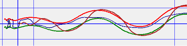
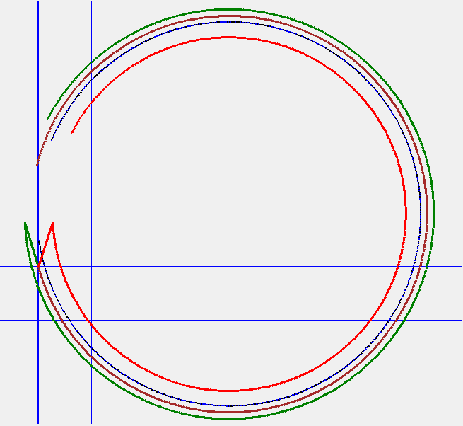
A Trikke needs a rider to drive it, even a simulated Trikke. Driving actions must be coordinated and actuated at appropriate levels to obtain locomotion. Though it was relatively easy to find productive driver configurations, it is a somewhat subjective matter to find one that behaves properly "expert". These experiments are driven by the digital Robot-Rider described in the paper on the computer [simulation]. A couple sets of these experments were actually performed with different robot-riders yielding slightly different results. They helped to weed out issues in the physics, simulation and resulting data presentations. Figure 1 shows a trajectory plot from the simulation. While validating and pretty, is not particularly enlightening. Raw data, graphs and charts are needed for that.
Variables and Factors
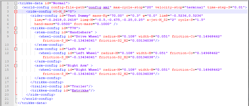
Scenarios can be run for endless variable configurations. The configuration file Figure 2 for a Normal simulation run has 33 of them! Three variables control how the simulation terminates. 15 variables control the rider and the initial Trikke speed. The rest configure the Trikke rider's body, wheel and friction profiles. Six of the run-configuration variables are the primary focus of this study. Variables that are not changed have either been set by actual geometry, indirect measurement or a guess based on other research or riding experience.
Input Limits: Each simulation configuration variable can be examined by itself, but the rest must provide a valid context. Leaning the steering column side-to-side may not make sense if the rider's center of mass falls beyond trailing arm boundaries. Most of the configuration variables occupy natural physical limits. How much angular thrust aσρ, a rider provides, how long a rider's drive cycle τ lasts and how quickly the rider turns σ are more subjective. An upper limit for aσρ is based on achievable terminal velocity. τ by experience. σ is constrained to be less than half of the drive cycle τ/2 less any Rest φ the rider may include.
Data Production: Depending on the simulation step size and termination conditions, each run produced a rather verbose XML data file about 4 MB in size, 40 MB the largest. Values include physical configuration, simulation control and dynamic data for each main model component. See [simulation]. Most of the graphs and other data representations in this study result from simulation data. The granularity of the results depend on a simulation step size. The smaller the step, the greater the detail, time and data volume. A Trikke usually travels less than five centimeters in one-hundredth 0.01 of a second. At this length-scale little happens too quickly for the simulation to expose. Setting the time step smaller verifies that kinematic variables converge well to the same values.
Termination: There are three different types of simulation termination. The method of termination does not affect the other configuration-variables of a run, unless it stops the simulation "early". Since it was not known what the best termination strategy would be before a run, it was often necessary to run a simulation more than once to allow the behaviors to complete. The configuration parameters "velocity-stop" and "max-cycle-stop" control termination. "velocity-stop" has one of three values shown in the list below. Regardless of the stopping mechanism, "max-cycle-stop" terminates the simulation at its specified number of cycles to avoid runaway processing. The length of a cycle is set by the value of rider-config/@cycle-S. The number of data frames generated in a cycle depends on time-step-S. At 1.5 seconds per cycle and a time step of 0.01 seconds, 150 data frames or steps are generated per cycle.
- velocity-stop="none" lets the simulation run for exactly max-cycle-stop cycles regardless of what the Trikke frame or cycle velocities are doing. This is typically used when the rider variables fail to produce any forward velocity at all or the velocity oscillates.
- velocity-stop="coast" terminates when frame-velocity is zero or less in the forward direction or after max-cycle-stop cycles. Normally used when there is initial velocity "v0-M_S" or "cruise" and the rider variables fail to produce sustainable forward velocity.
- velocity-stop="terminal" terminates when cycle-velocity is within a millimeter per second of the previous cycle; terminal velocity has effectively been reached. Cycle-velocity is the average cycle speed. Used when the rider variables produce viable speed, usually starting from a stop.
The main input variables to the Trikke simulation are presented in Table 1 below.
| Variable | Description | Units | Range | Neutral |
|---|---|---|---|---|
| v0 | Cruise†: Initial speed of the Trikke. Alternatively called coasting when expected to end with no velocity. | meters per second | 0 9 (20 mph) | 0 |
| θ | Steer: Steering column turn angle limits. Note that Caster is Steer and Camber together. | radians | -π/2 π/2 (90°) | 0 |
| γ | Camber: Steering column vertical angle limits. Thia action completes in half a cycle less rest. Caster is Steer and Camber together. | radians | -0.2618 0.2618 (15°) | 0 |
| ψx | Sling†: Rider's center of mass position (Cm.x) x-axis limits; fore and aft. Note that Push is Sling and Lean together. | meters | -0.5 -0.85 | -0.5 -0.5 |
| ψy | Lean*: Rider's center of mass position (Cm.y) y-axis limits; across the Trikke. Push is Sling and Lean together. | meters | -0.25 0.25 | 0 0 |
| aσρ | Jet†: Upper limit of body rotation jet-acceleration measured as linear acceleration at the guide-wheel contact point. Carving is Push and Jet together. Can be tuned to Cycle to keep maximum velocity at a constant value. aσρ = vmax/((0.5 - σ/2 - φ) τ) | meters per second-squared. | 0 6 | 0 |
| σ | Punch*: Interval during which θ steers from one limit to the other. | cycles | 0 0.5 - φ | 0.3 |
| φ | Rest†: Interval during which the rider applies no change in Steering or Camber and engages no carving inputs; Jet, Sling nor Lean. | cycles | 0 0.5 - σ | 0 |
| τ | Cycle: Rider's drive cycle time. Usually includes steering one way then the other coordinated with momentum transferring mechanisms. | seconds | 0.5 3 | 1.5 |
| w | Mass: Rider's mass. | kg | 60 90 | 70 |
Who comes up with theses names rendered in bold style? Designations for these variables are inspired by terms used in the *Trikke community and some are †my suggestions. It is more than likely some will not agree with their precise semantics. Of all the possible monikers, I believe these serve best. "Cruise", "Sling" and "Jet" are my contribution to the colorful, yet mathematically well-defined terminology.
Can even the most experienced, disciplined, body-powered/fitness Trikke rider command these variables independently in real-world rides? Not likely. And if one could, video and difficult analysis are the only way to verify the performance. Without a precise framework like the simulation, there is little purpose in trying to define these terms too tightly. Several times, I thought I was applying one riding strategy only to find later it was likely something more subtle. Never-the-less this study as well as the others benefited from a near daily cycle of research, theory and rides trying to apply what I learned. Part of that effort resulted in the digital Trikke riding robot Figure 3 that is capable of precise execution of each variable independently.
If each of the ten variables were set in unique combination with the others using only their extreme limit values, an exhaustive 2-Level screening technique, there would be
to run. Some of those 1024 would not be meaningful, except to verify that the simulation produces no false results. Neutral and coasting-only scenarios where nothing changes once under way serve this verification purpose. About half of the 1024, those with no steering, would likely result in no attained forward velocity as steering is known to be essential in Trikke locomotion.
Determination of Trikke Behavior
Defining input parameters allows all kinds of experiments to be defined and performed. Even in virtual experiments like those that follow, one or more input factors is varied in a suite of configurations. When executed, the simulation measures many aspects of the process under study. Those configurations that show variation in behavior help expose the sequence and mechanisms that the data represent. As a Trikke rider interested in the "best" ride for the least input energy, the dependent measurements must provide information about:
- Input and output energy profiles
- Dynamics of the Caster-Pull and Push mechanism
- Dynamics of Carving mechanism Jet and Push which involves Sling and Lean
- Role of friction and inertia
- Path measurements like trajectory, swath and stride
- Coasting behavior, especially compared to the empirical study
- Behavior while accelerating to terminal velocity
Such measurements include familiar kinematic data like acceleration, speed, distance and some not so familiar like path trajectory and swath. Since rotation is so important to riding a Trikke angular acceleration, speed and distance may play a part. Dynamics include masses, inertial mass, moments of inertia, leverage, force, stride and various traces of internal and external variables sometimes plotted against their own components as hodographs.
Below virtual experiments are preformed that collect much of this kind of data for analysis and interpretation.
- Trikke Behavior at Terminal Velocity
- Design of Experiment: Screen and Model
- Cycle, Punch and Mass Factors
- Simulated Coasting vs. Measurement coasting results with those in the Friction analysis measurements.
- Single Factor Cruising.
- Effect of Steering on Carving Profile θ in normal Caster Carve
- Jetting to Attain a Specific Speed
- Varying Punch
- Effect of Rider Weight on Speed
Here are some common considerations in the presentation of these experiments below:
- Each input has a valid operating range; presented in Table 1 above.
- Each scenario highlights the subject variables in bold. These have values that differ from the "Neutral" or control scenario defined for each experiment.
- When multiple variable values are listed in a scenario, they indicate related runs of the same configuration.
- Two numbers in a cell indicate the limits for the robo-driver to execute according to its periodic driving algorithm described in the [simulation] paper.
- Stop conditions specify how the simulation was terminated. As mentioned above, this often required more than one run of the scenario.
The first experiment is essentially a "control". It's not so much of an experiment as it is a means to become familiar with Trikke mechanisms and some ways of representing their simulated output. Being more or less familiar with "normal" helps to identify what is not. Those are the sorts of things that require explanations and exercise our understanding for application later on to goals like "better riding technique".
Trikke Behavior at Terminal Velocity
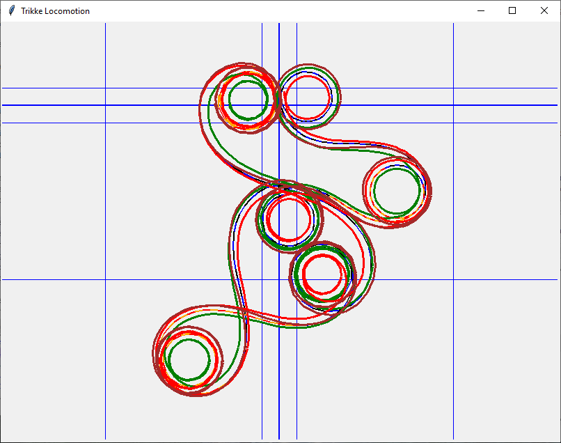
The first behavior to look at is "normal". What is a normal Trikke ride? Of course, any real-world ride is much more interesting than one constrained to a simulation. But there are actually few constraints on the simulation in terms of how the ride develops. Figure 4 to the right shows simulated wheel trajectories with an unreasonably high Jet value. Most normal simulation runs snake along a delicately balanced, straight swath as the expanding one in Figure 1 above. Intentionally turning by setting steering with a bias produces circles as in Figure 24 below, but that is not necessary to produce normal behavior.
A normal Trikke ride begins at rest and accelerates to a terminal velocity which the rider attempts to maintain for the duration of the exercise. However once terminal velocity is achieved, the simulation provides no more interesting information; it just repeats the terminal cycle spitting out the same data endlessly. Normal introduces us to reasonably good Caster and Carve, the weak involuntary and the strong intentional momentum transfer mechanisms of a Trikke. Further along in this paper, a simulation configuration known as "DoE 2**5 configuration 15" produces the conditions for extreme Caster Carve. It's difference from Normal is that Sling ψx = -0.85 m and Jet aσρ = 2.666 m/s2.
Normal Configuration factor values:
w = 70 kg, θ = 30°, γ = 15°, ψx = -0.675 m, ψy = 0.25 m, aσρ = 2 m/s2, v0 = 0 m/s, τ = 1.5 s, σ = 0.3, φ = 0
Note, the simulated rider weighs in at 70 kg, about the author's mass. This mass is used in all these simulated configurations except the experiment that determines the effect of a rider's mass on performance. To understand the various physical mechanisms discussed below, see the paper by this author on Trikke [physics]. The Glossary also contains general information about some typical Trikke terms like carving.
Terminal Input Energy Profile
How is input energy distributed among the various input factors over typical cycles?
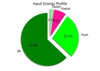
Figure 5 shows the input energy distribution during a cycle at terminal velocity of the Normal Caster Carve configuration. Greenish areas represent input that can drive the Trikke, while reddish areas represent processes that require energy to create the green drive energy. The green region covering 62.9% of the pie represents how much Jet energy rotated into the locomotive effort. To expend 27.5% of the input energy pushing the Extended-Trikke, the Rider inadvertently dumped 7.5% of the input energy into radial friction at the wheels due to misalignment of movement and the path. 2.1% of the input energy went into castering. These input energies are apportioned based on energy conservation on an arched trajectory as detailed in Trikke [physics].
I was really surprised by how tiny castering input turned out to be and how large jetting was. As my riding improved, my arms relaxed much more and didn't feel like they were going to fall off anymore. This rider recoil from pushing and feeding the caster mechanism must equal the sum of the radial waste, push and caster input. Learning to make these motions efficient took time. Radially directed momentum produces the transverse wheel constraints that keep them rolling straight. If too strong, though they can slip! Pushing in harmony with the motion of the Trikke enables me to guide the acceleration it creates and to eliminate the center of mass reset pull.
The input pie is largely stationary over the course of a simulation run since the robot produces the same input patterns each cycle but the first. Initially, the guide-wheel points straight ahead and is turned through only half a "sweep" to the left in the first half-cycle. Configurations without jet are quite different as the area it occupies in this pie is filled in by the other input factors.
Average energy input at terminal velocity for the Normal configuration is about 340.6 J per second. That's 340.6 W (power). Just breathing and awake, a person expends about 100 W. Exercising with a Trikke in the Normal way at 340.6 W for an hour burns
Terminal Output Energy Profile
How is output energy distributed among the various forms of output variables over typical cycles?
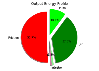
Figure 6 shows the output energy distribution during a cycle at terminal velocity of the Normal Caster Carve configuration. Again, greenish areas represent driving outputs, while reddish ones represent "wasted" energy. The green region covering 37.3% of the pie represents how much Jet energy pushed the guide-wheel along its path. It was opposed by 50.7% (red) of the output energy dissipated in friction, heat, vibrations and sound. In addition to friction, wheel inertia output of 0.6% opposed the Trikke's progress. Direct-push resulted in 10.1% of the output energy pushing the Trikke. 1.3% of the output energy came from caster-push. Driving energy vs. opposing energy is 1.3% from equal. At terminal velocity, half the output energy creates movement and half opposes it.
Output energy distribution changes rapidly each cycle when starting from a stop. In cycles accelerating to terminal velocity, friction and inertia (storing energy in the wheels) do not yet equal the green areas. It settles to a constant state at terminal velocity, with friction plus inertia equal to everything else added together. Configurations with no Jet fill in the pie chart area with the remaining mechanisms. If a run fails to move the Trikke, the output pie can be completely red and pink. Note also, output inertial energy for coasting is an aid to movement as energy stored in the wheels is released.
Average energy output shown in the corresponding pie chart is lower at 206.3 J per second. That's 742.7 kcal by the same accounting as above. Note that at terminal velocity, half of the output energy necessarily goes into friction and its various forms of drag. So the actual motive output is half: 103.15 J. Trikke Efficiency is the measure of input energy required to attain motive output energy.
Terminal Caster Data
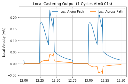
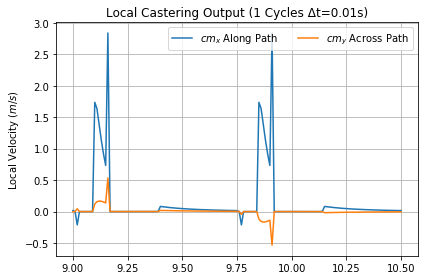
Whenever the handlebars are turned, the Trikke casters. Beginning from the limit of a turn, the caster offset pulls the yoke across the stem until the guide-wheel points forward. During this time, the trailer rotates around the transom point into the turn powered by the rider's arms. Continuing the turn to the other side, this caster angular momentum transfers as jet impulse to the TRS at the guide-wheel contact point. Figure 7 shows the extra guide-wheel velocity developed via caster during a cycle at terminal velocity. In the forward component (blue) there are two waves, one for each half cycle.
Note the two peaks in each half cycle wave. During the first part of each half-cycle, there is no caster velocity at all while the trailer gains angular momentum. The initial rounded spike shows energy transfered during the turn past forward until camber passes vertical. At this point in the cycle, the transom point moves quickly beyond the center line allowing more angular momentum to transfer until steering stops. When the rider and transom point reach their side-limit, Camber continues to move the yoke further into the turn creating the low curve at the end of the half-cycle. The across-path component (orange) is much smaller, but follows a similar pattern. For the across path or y-axis curves, positive values above the zero-line are on the left and negative are on the right. Caster is proportional to Punch input.
Terminal Carving Data
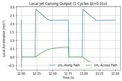
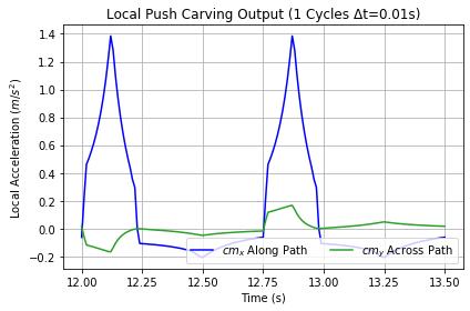
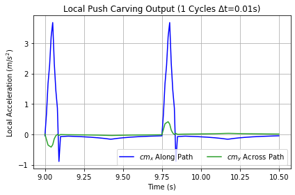
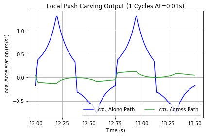
Carving consists of a rotation component of Jet and a direct-push component of Push. Push results from Sling along the guide-wheel path and Lean across the path. The two graphs below in Figure 8 and Figure 9, show Jet and Push respectively over a cycle at terminal velocity. Jet input velocity in this scenario rose linearly from 0 to 1.5 m/s as shown by the orange curve in Figure 3. The simulation provides the average increases in local coordinate frame acceleration which are approximated in Figure 8. There is no jet until after the turn rolls out straight. If there was, it would be in the opposite direction, so the robot avoids it altogether. Note the acceleration along the path (blue) falls linearly from 2.86 m/s2 until the turn ends. Then it is about 2.2 m/s2 until the next turn starts. Across path acceleration (green) is significantly less. Adding the components together produces a constant total acceleration of 2.86 m/s2, which is consistent with the 0 to 2 m/s robot input.
Figure 9 Shows along path and across path acceleration due to push. Push motivates from shifting the rider's center of mass cmx along the path (Sling in blue) and across the path cmy (Lean in green) in the figure. For the across path or y-axis curves, positive values point to the left and negativepoint to the right. The generation of Push is more complicated than jet. While turning from the initial right-hand limit to the center, forward push builds and reaches its climax when the rider moves backward quickest. Forward acceleration crashes after passing straight while turning to the left. The robot has not been programmed to completely avoid the restoring pull, but it is much smaller than the push. As the robot-rider moves forward to reset position for the next push, the guide-wheel contact is decelerated a small amount. When the rider is not shifting weight, Push has zero velocity. Note that the output Push accelerations are about seven times the castering accelerations at Normal half-maximum Sling. Push rises much higher with maximum Sling.
|
|
Friction Data While Accelerating
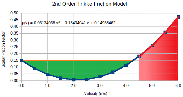
An empirically [calibrated] 2nd order Friction Model apportions friction forces to each wheel contact patch in the simulation. Figure 10 on the right shows friction vs. velocity for a T78-Air Trikke I ride. The scalar model coefficients shown in the equation on the chart are used for each wheel in the simulation. Note the minimum at 2.1432 m/s (4.8 mph). Multiplying the minimal friction coefficient by Trikke+Rider load (g 82.65 kg) gives 4.64 N. If Cruise is set to 2.2 m/s, input resulting in about 5 Newtons of continuous output force should sustain the cruise at or above 2.2 m/s, otherwise, it coasts to a stop. While on the subject, using the same calculation, notice it takes about 122 N to get the Trikke moving (green) and more to reach higher terminal velocities (red).
Eqn 1: μ(v) = 0.14968462 - 0.13434041 v + 0.03134038 v2
where μ(v) is the modeled scalar friction coefficient and v is the velocity of the contact.
Eqn 2: Fμ = L g μ(v)
where L is the load on an axle in kg, g acceleration of gravity.
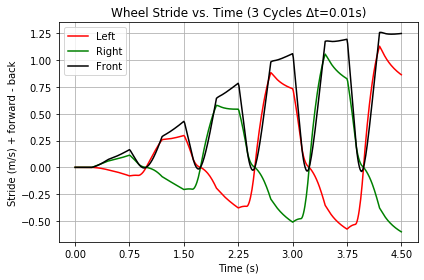
Wheel stride is the difference between the center of mass velocity and that of a wheel. Figure 11 on the right shows stride for each Trikke wheel in the Caster Carve configuration speeding up to terminal velocity. Note that the left (red) and right (green) wheels actually travel a little slower than the center of mass each cycle on the inside of turns. On the outside, they travel almost as fast. The guide-wheel (black) dips to zero when traveling forward, otherwise is faster than the rear outside wheel. When the Trikke travels at 1 m/s, the front wheel and outer trailing wheel may be traveling at 2.25 m/s where the friction coefficient is very low as shown in Figure 10 and the inside wheel is at an even higher value on the curve than the center of mass would be. A rider wanting to take advantage of this stride geomerty should somehow load up the front and outer wheels at that time in the cycle to reduce friction. Once the Trikke's center of mass attains 2.5 m/s, such a strategy would slow it down! Stride changes with steering limits and Punch.
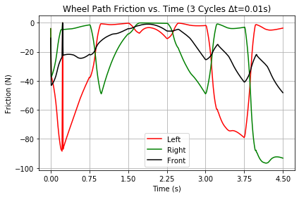
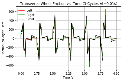
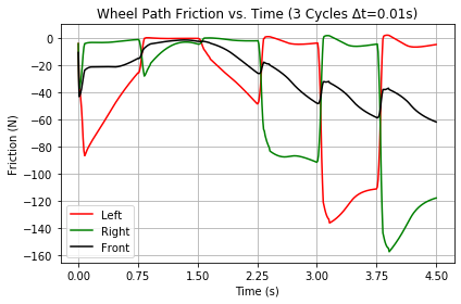
Figure 12 shows how well the robot-rider did in terms of friction force along each wheel's path and across it in Figure 13 accelerating from a stop for three cycles. The first cycle begins from center turning left. After that, each cycle begins at the right turn limit and starts turning to the left. That initial turn to the left produces a relatively large amount of forward friction. Friction almost evaporates in the second 1.5 second cycle, then becomes more typical in the third cycle with the inner wheel loaded up and the outer practically weightless.
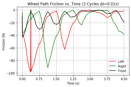
Transverse friction in Figure 13 includes the rider's radial push component that depends on the rider's local trajectory and position relative to the guide-wheel contact point. Though dependent on the rider's center of mass angular displacement, all three wheels seem to take on about the same amount of friction, about five times the forward values. In this graph, positive values indicate friction to the left and negative to the right. Initially, the deceleration from friction radiates to the inside of the turn on the left side. If the wheel slips it slides outward with the motive force, against diminishing friction. Friction is greatest on the left until the rider's full weight is near the left wheel. Pulling begins as the rider resets to carve to the other side. With the pull, friction switches sides. The pull is smaller than the push, but it aligns better with the path and attains a similiar opposite shape in the graph. When the pull stops, friction jumps to the left to oppose the last bit of jetting before the next turn. This is the pattern followed each half-cycle.
Doesn't the friction on all wheels add up to the same overall friction force? It would if the model was linear. It is not! But beware, as the center of mass speed passes 2.2 m/s, the outside wheels take on higher friction coefficients than the inside wheel! Now the rider should load up the inside wheel that has the lower value.
|
|
Design of Experiment (DoE): Screen and Model
This discipline is a type of designed experiment contrived to efficiently screen for main effects and model the effects of several factors against each other using Yates analysis. It attempts to optimize measurable differences in output effects and minimize the number of trials to obtain them. When models are obtained they have least-squared multilinear properties subject to the confounding structure of the experiment. When the resulting models do not represent the experimental data, the true model must be non-linear. Typically, replications of the experiment are performed and Analysis of Variation determines confidence intervals for each factor effect. The DoE experiments presented here cannot be run in the Real-world as no Trikke rider can perform the necessary independent input maneuvers. Since the simulation has no ability to simulate system error propagation it produces data without replication or random variation.
Four DoE experiments were run. First a Fractional Factorial DoE Screening 2**(6-2)IV design with 16 configurations (un-replicated) showed that Steer θ had the greatest effect, but the model was non-linear. Simulation vs. multilinear model produced a residual standard deviation of about 0.5 m/s. With average terminal velocities of about 1.5 m/s, that's a terrible model! Leaving Steer out enabled a simple 2**(5-1) Fractional Factorial Design with 16 configurations. 7 of the configurations were common to both of these 2-Level experiments. Results showed a "perfect" model, but the confounding structure is intuitively contradictory "equating" configurations that surely produce very different results. The only way out of having to explain these impossible equality classes was to perform the full 5 Factorial Design with 32 configurations. The final DoE study includs Cycle, Punch and Mass in a full 2**3 design.
These DoE studies, especially the last two, which appear in this article, provide a back drop against which to interpret the more directed experiments that follow.
The factors that a rider uses to produce locomotion have different units and ranges. One might think cambering should have a large effect since the rider has to move the stem quite far each cycle. On the other hand, it is difficult to see the effect of jetting since it's hard to know what is twisting and in which direction. In Yates Analysis, comparison of effect begins as each factor's extremes are "Normalized" between -1 and 1. The genius of Yates Analysis is that once factor input values are normalized, the effects are as well. This "Code" method makes it possible to work with an n-dimensional cube-shaped factor space and allows the construction of a multilinear predictive model with least-squares optimization properties.
DoE Full 2**5 Factorial Design with Camber, Sling, Lean, Jet and Cruise
In every configuration, each simulation factor is set to its corresponding -1 or 1 code value, depending on whether it should be a minimum for the factor or a maximum. The minimum configuration values constitute the Neutral configuration; all factors are set to their corresponding -1 values. However, since steering angle θ is not one of the factors in this modeling study, it is set to θ = 0.5236 radians (30°). The other factors studied in another DoE study below are Cycle at 1.5 seconds, Punch set to a phase of 0.3 cycles and Mass at 70 kg. Rest is the final factor set to 0 cycles. Table 2 shows the five factors of this study, their normalizations and extreme values.
| Factor | Conversion Expression | -1 (Low) | +1 (High) |
|---|---|---|---|
| Camber | γc = (γ - 0.1309)/0.1309 | 0° | 0.2618 rad (15°) |
| Sling | ψxc = (-ψx - 0.675)/0.175 | -0.5 m | -0.85 m |
| Lean | ψyc = (ψy - 0.125)/0.125 | 0 m | 0.25 m |
| Jet | aσρc = (aσρ-1.905)/1.905 | 0 m/s2 | 3.810 m/s2 |
| Cruise | v0c = (v0 - 2.01168)/2.01168 | 0 m/s | 4.02336 m/s (9 mph) |
Low coded values are neutral values. In the case of Camber and Lean, the values actually "sweep" over the range of values from minus the coded value to its positive over the course of a cycle. Camber of 15° is fairly steep, but close to my prefered action as a rider. Sling sweeps from -0.5 to the coded value. The extreme values for Sling and Lean are close to the physical limits a rider can occupy safely on a Trikke. While possible for a rider to attain, these are not likely limits a rider would pursue for long - it's a lot of work.
A jet of 3.810 m/s2 with near maximum Sling accelerates the Trikke to about 4.9 m/s (11 mph) in just over three cycles. Sticking to a precise input regimen, the simulation is a bit unrealistic. A real rider finds it difficult to control initial Jetting and Slinging so well. Settling into a harmonic rhythm at speed smoothly shifts the rider's momentum to the Trikke. Without the "set up" from a previous cycle, it is a struggle to coordinate motive efforts when starting a Trikke from a stop. As a result, a real rider takes a couple more cycles to get up to speed.
Cruise extremes are reasonable speeds most Trikke Riders can likely muster.
and Cm "wobble"
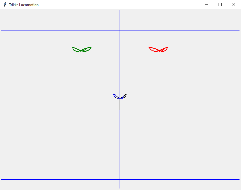
All 32 configurations for the simulation factors are shown below in Table 3. Terminal velocity (vt) of the Trikke-Rider System TRS, technically "forward speed", is the result used to determine whether or not the Trikke-rider experienced locomotion. In several of the configurations, there is TRS center of mass motion following a closed trajectory for some distance (like side-to-side wobble), but the guide wheel does not progress forward, vt = 0. See Figure 14 for example. The guide-wheel makes contact at the intersection of the meter lines at the bottom.
Please refer to the experiment design Table 3 below. The names of the +1 factors and their combinations identify each configuration. Terminal velocity vt of the run is recorded. The non-coded factor symbols are used to indicate that non-coded values corresponding to the coded values indicated below were used to configure each run. Stop conditions are noted. It often took a couple of simulation runs to establish correct termination conditions.
| Configuration | vt | γc | ψxc | ψyc | aσρc | v0c | Stop Condition |
|---|---|---|---|---|---|---|---|
| 0 Steer Only | 0.0000 | -1 | -1 | -1 | -1 | -1 | 5 cycles |
| 1 Caster Only | 0.0000 | 1 | -1 | -1 | -1 | -1 | 5 cycles |
| 2 Steer Sling | 0.0000 | -1 | 1 | -1 | -1 | -1 | 5 cycles |
| 3 Caster Sling | 0.0000 | 1 | 1 | -1 | -1 | -1 | 5 cycles |
| 4 Steer Lean | 0.0000 | -1 | -1 | 1 | -1 | -1 | 5 cycles |
| 5 Caster Lean | 0.0000 | 1 | -1 | 1 | -1 | -1 | 5 cycles |
| 6 Steer Push | 0.0000 | -1 | 1 | 1 | -1 | -1 | 5 cycles |
| 7 Caster Push | 0.0000 | 1 | 1 | 1 | -1 | -1 | 5 cycles |
| 8 Steer Jet | 4.9833 | -1 | -1 | -1 | 1 | -1 | Δv = 0 or 20 cycles |
| 9 Caster Jet | 4.9794 | 1 | -1 | -1 | 1 | -1 | Δv = 0 or 20 cycles |
| 10 Steer Sling Jet | 4.9797 | -1 | 1 | -1 | 1 | -1 | Δv = 0 or 20 cycles |
| 11 Caster Sling Jet | 4.9794 | 1 | 1 | -1 | 1 | -1 | Δv = 0 or 20 cycles |
| 12 Steer Lean Jet | 4.9572 | -1 | -1 | 1 | 1 | -1 | Δv = 0 or 20 cycles |
| 13 Caster Lean Jet | 4.9601 | 1 | -1 | 1 | 1 | -1 | Δv = 5 cycles |
| 14 Steer Carve | 4.9596 | -1 | 1 | 1 | 1 | -1 | Δv = 5 cycles |
| 15 Caster Carve | 4.9572 | 1 | 1 | 1 | 1 | -1 | Δv = 0 or 20 cycles |
| 16 Steer Cruise | 0.0000 | -1 | -1 | -1 | -1 | 1 | v = 0 or 20 cycles |
| 17 Caster Cruise | 0.0000 | 1 | -1 | -1 | -1 | 1 | v = 0 or 50 cycles |
| 18 Steer Sling Cruise | 0.0000 | -1 | 1 | -1 | -1 | 1 | v = 0 or 50 cycles |
| 19 Caster Sling Cruise | 2.2779 | 1 | 1 | -1 | -1 | 1 | Δv = 0 or 50 cycles |
| 20 Steer Lean Cruise | 2.6324 | -1 | -1 | 1 | -1 | 1 | Δv = 0 or 50 cycles |
| 21 Caster Lean Cruise | 2.7220 | 1 | -1 | 1 | -1 | 1 | Δv = 0 or 50 cycles |
| 22 Steer Push Cruise | 2.8424 | -1 | 1 | 1 | -1 | 1 | Δv = 0 or 50 cycles |
| 23 Caster Push Cruise | 2.9014 | 1 | 1 | 1 | -1 | 1 | Δv = 0 or 50 cycles |
| 24 Steer Jet Cruise | 4.9528 | -1 | -1 | -1 | 1 | 1 | Δv = 0 or 50 cycles |
| 25 Caster Jet Cruise | 4.9490 | 1 | -1 | -1 | 1 | 1 | Δv = 0 or 50 cycles |
| 26 Steer Sling Jet Cruise | 4.9497 | -1 | 1 | -1 | 1 | 1 | Δv = 0 or 50 cycles |
| 27 Caster Sling Jet Cruise | 4.9404 | 1 | 1 | -1 | 1 | 1 | Δv = 0 or 50 cycles |
| 28 Steer Lean Jet Cruise | 4.9262 | -1 | -1 | 1 | 1 | 1 | Δv = 0 or 20 cycles |
| 29 Caster Lean Jet Cruise | 4.9293 | 1 | -1 | 1 | 1 | 1 | Δv = 0 or 50 cycles |
| 30 Steer Carve Cruise | 4.9292 | -1 | 1 | 1 | 1 | 1 | Δv = 0 or 50 cycles |
| 31 Caster Carve Cruise | 4.9270 | 1 | 1 | 1 | 1 | 1 | Δv = 0 or 20 cycles |
| Average | 2.8948625 |
These 32 configurations and their velocities can be grouped in the following ways. Eleven of the runs resulted in no locomotion. Sixteen of the runs attained 4.9 m/s (11 mph). Five were between 2.2 and 3.0 m/s near the average 2.895 m/s (6.5 mph). This overall average is a bit above the speed at which friction of the Trikke is lowest 2.2 mph. Such extreme results were not expected. Also notice that configurations in 8 to 15 had non-zero terminal velocities that were slightly higher than their Cruise counterparts in configuration 24 to 31, most just over 3 centimeters per second. Equality was expected as Cruise does not affect the dynamics once the run has begun. However, the Cruise enhanced configuration runs converged to terminal velocities in only 5 cycles; half that needed for the lower numbered configurations! They were already traveling just under their terminal speeds.
With Cruise added, Steer Only, Caster Only and Steer Sling still coasted to a stop. Configurations 3 to 7 stopped, but they all achieved low terminal velocities when Cruise v0 was added in 19 - 23. All of the configurations that stopped or had low terminal velocities did not include Jet. The five with low terminal velocities coasted down to speeds slightly above that of the friction minimum velocity. The non-linear friction model accounts for this. Starting from a stop much more friction has to be overcome to speed up enough to get to the lower part of the friction curve. If it can't get there, friction defeats the motion in a weak part of the drive-cycle. With 4 m/s Cruise, the Trikke starts out just under the friction needed to propel the Trikke from a stop. If the robot is not producing enough locomotion to sustain that level, the Trikke slows down until it matches friction at a lower speed. If it can't out perform or match minimum friction at 2.2 m/s, then it grinds to a halt. Starting from Cruise greater than or equal to 2.2 m/s gives it two chances to find a terminal velocity.
Figure 15 shows the next step - determining the main effects via a Pareto chart. In many cases about 80% of an event's effects come from 20% of the causes. This is the Pareto principle, named for the Italian economist who promoted it with charts like this. A 2**5 design (two levels +/-1, 5 coded factors γ ψx ψy aσρ v0) produces 31 effect coefficients, one for each unique multilinear factor combination. 16 of them are negative effects. These detract from locomotion and are excluded from the figure and red-line totals. After sorting, bars are plotted in descending order. The red line is their running total up to 100%. Normally at this point, Analysis of Variance determines which effects are significantly higher than the others. But as mentioned, the simulation has no means of error propagation, so there is no variance in the results to analyze.
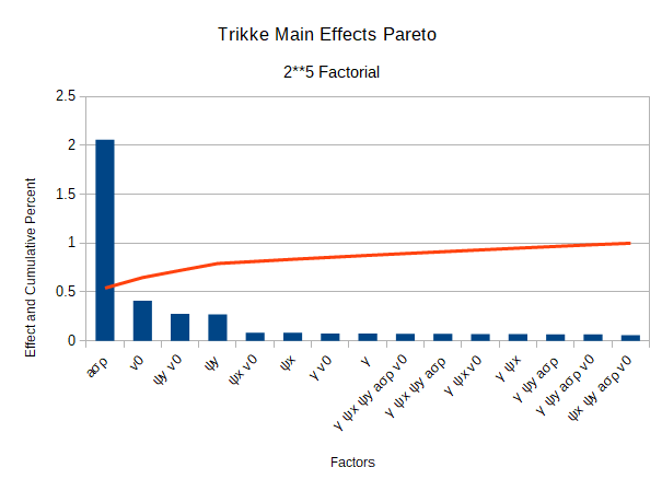
There are 32 effects, each a coefficient of one or more factors (multilinear term) except the first, which is the average of all the resulting vts. Each factor shows up in 16 multilinear terms. Each appears in 7 of the positive, Pareto terms, except Jet, which shows up in 6 terms and Camber, which shows up in 8. All multilinear terms also have Steer by default since locomotion doesn't happen without it. Steer Jet and Steer Cruise top the list, but all 5 factors show up with Steer as positive effects. Next with the same effect are Steer Lean Cruise and Steer Lean. Steer Sling Cruise and Steer Sling are next followed by many multilinear factor combinations with similar effects. They are so close in value that order does not matter. One cannot say that Steer Sling has more effect than Caster (Steer Camber) or any of the multilinear terms. Generally, if a term has a positive effect, the +1 values of its factors contribute more to the final configuration velocities than the -1 values degrade them. Similarly, a negative effect indicates the -1 values combine to bring the final velocities down more than the +1 elevates them. Larger magnitude negative terms like Steer Jet Cruise, Steer Lean Jet and Steer Lean Jet Cruise have matching trial configurations with terminal velocities at the lower end, but stll over 4.9 m/s. All of the coefficients show up in the terminal velocity coded model equation in Figure 18.
Jet has by far the most effect on Trikke locomotion, but that does not mean riding by only steering and jetting is the best technique. Steer Jet, configuration 8, produced the highest terminal velocity at 4.9833 m/s. Adding in singly or in combination any of the other factors detracts from the performance of this configuration. Camber and Lean detract the most as evidenced by configurations 12 and 15.
Adding in Sling makes the Steer Sling Jet configuration which has the next highest terminal velocity. Sling causes a direct push and a direct pull. Because there is no rider Lean to dump pull in radial waste, the pull slightly more than cancels the push. Therefore the reduced terminal speed.
Adding in Camber gives the Caster Jet configuration. This owns the next best terminal velocity. Camber Effectively speeds up the guide-wheel contact velocity by lengthening its transverse path. This increases the stem turn-radius without changing the TRS center of mass turn-radius. This lowers the Jet's mechanical advantage slightly. Adding in Sling into Caster Jet does not alter vt (ref. Caster Sling Jet). Camber helped in some cases as attested to in the Steer Sling Cruise vs. Caster Sling Cruise, the Steer Lean (Push) Cruise vs. Caster Lean (Push) Cruise and configurations 28 and 29. There are also many such configuration pairs where it detracted from vt. However, the pluses counted more than the minuses and so Camber has a slightly positive effect.
Adding in Lean matches the Steer Lean Jet configuration which has a little lower terminal velocity. Lean causes more momentary load on the faster outside wheel. Since it has more friction than before, it reduces the terminal speed. When riding fast, I tend to throw the Trikke from side-to-side while twisting around my fairly stationary z-axis in the center. I suspect the outside wheel still loads up a bit. Oddly, adding to this Camber and Sling does not change the terminal velocity (ref. Caster Carve).
Lastly, adding Cruise to Steer Jet results in Steer Jet Cruise. This configuration is a little slower than the others mentioned so far, but is the top Cruise configuration. The results clearly show that adding Cruise to any configuration reduces its terminal velocity at least 3 cm/s. With Cruise added the configuratons mostly maintain the same speed order. Why the slow-down? Cruise starts the Trikke at a speed just under the eventual terminal velocities. It takes only 5 cycles to get there; about half the number needed from a stop.
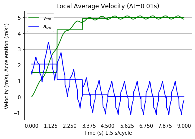
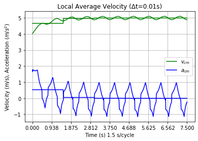
Steer Jet θ aσρ clearly has the highest input-to-output effect. Steer is included in the name and symbol because none of these factors have an effect without it. Had a lower "extreme" value been used, the jetting effect would not be as high, but it would likely still be the highest one. The Jet factor value of 3.810 m/s2 was chosen because it was known to produce reasonable Trikke speeds, but not maximum; even for this rider. Jetting makes the Trikke go! Figure 16 below plots the velocity (green) and acceleration (blue) of the Trikke and their cycle averages until terminal velocity is achieved.
|
|
With cruise, Steer Jet reached vt 4 cycles faster than with out Cruise; see Figure 17. However, the plot in Figure 17 does not match the part of Figure 16 following v = 4 m/s as it would in coasting. Because of steering alternately to each side, it reaches vt in a slightly different way. The selected Cruise velocity 4 m/s does not occur at the beginning of a cycle for the configuration that starts from a stop. It appears to occur at 2.25 cycles in Figure 16 rather than at the beginning in figure 17. They are out of phase! However one or two cycles later, they are back in phase, but the coasting velocity average is a little lower. Since this occurs in all of the Cruise configurations which had viable non-Cruise configurations, I suspect that the Cruise runs' velocity average migrates upward more slowly than 1 mm/s which triggers vt termination. Given enough cycles, they would eventually match.
Never-the-less, if Cruise reduces the speed of configurations, why is it the factor with the second greatest positive effect? Note that configurations 0 to 7 had no accumulated speed at all. While Cruise detracts 3 cm/s from speedy runs, it adds over 2.2 m/s to 5 of the no go runs. Overall, it's a winner. Note these configurations can not struggle from a stop to gain speed. But once moving, the friction is low enough for 5 of them to settle into stasis. These configurations involve Push components with or without Camber. As implemented by the robot-rider, Sling by itself provides direct push and a somewhat less pull for a longer time. In total, the push is just a little larger, but too weak to overcome a stop. Likewise, Lean produces some push and somewhat less pull, but overall, a bit more than Sling. This can all change with different robot instructions Slinging and Leaning in a different way. But for this robot-rider and Cruise - "It takes speed to gain speed".
Steer Lean and Steer Lean Cruise have equal effect for this robot. Again, these factors separately and together seem to decrease terminal velocities for configurations that already have good speed. Note that Steer Cruise and Caster Cruise have no accumulated velocity. Add Lean to get Steer Lean Cruise and Caster Lean Cruise, both over 2.6 m/s. This seemingly small act of kindness no doubt earned Lean the spot. Similarly for Steer Lean Cruise, note configurations 2 and 3 have no resulting speed and no Lean or Cruise. With them, they become configurations 22 and 23 over 2.8 m/s each, another winner.
Coded Multilinear Model
One of the marvels of Yates Analysis is that the average output value and all the effects can be used to create a multilinear model with their respective coded factors! Figure 18 shows the resulting model. It took about two years to derive the physics, calibrate the friction and polish up the Trikke simulation. In about an hour and 32 simulation runs, it might all be replaced by this relatively simple equation if it passes one test! Of course it can't cover everything the simulation does, but the thought is outrageous.
Each of the 32 terms appears in multilinear factor order. The first term is the average of all configuration terminal velocities. This is a coded model. The factor symbols must be substituted by coded (normalized) factor values. It is possible to substitute in the normalizing equations, multiply out all the terms then collect in terms of the "real" multilinear factors. The result has the same form as the coded model, but all the coefficients are changed and unrelated to their factor's effects. It still requires a computer program to encode and execute the model, so not much is gained in the exercise.
vt = 2.8948625 + 0.07533125 γ + 0.08288125 ψx + 0.2703875 ψy + 2.05885625 aσρ + 0.41011875 v0 + 0.0698375 γ ψx - 0.06595625 γ ψy - 0.076325 γ aσρ + 0.0755625 γ v0 - 0.05853125 ψx ψy - 0.083825 ψx aσρ + 0.0831375 ψx v0 - 0.28088125 ψy aσρ + 0.27586875 ψy v0 - 0.4258875 aσρ v0 - 0.0724125 γ ψx ψy - 0.07061875 γ ψx aσρ + 0.06994375 γ ψx v0 + 0.067125 γ ψy aσρ - 0.06625 γ ψy v0 - 0.07609375 γ aσρ v0 - 0.058725 ψx ψy aσρ - 0.058725 ψx ψy v0 - 0.08356875 ψx aσρ v0 - 0.2754 ψy aσρ v0 + 0.07186875 γ ψx ψy aσρ - 0.07185625 γ ψx ψy v0 - 0.0705125 γ ψx aσρ v0 + 0.06683125 γ ψy aσρ v0 + 0.05930625 ψx ψy aσρ v0 + 0.072425 γ ψx ψy aσρ v0
How do we know if the coded multilinear model is any good? Table A-1 in Appendix A shows again each of the 32 configurations and the simulation terminal velocity result. It also shows the coded model results and the difference between the simulated result and its own; the residuals. They are pretty close, less than 3% error with a standard deviation of 8 cm/s. At the bottom, the averages are the same to 7 decimal places and the residuals average to nothing. Half of the residuals deviate by less than a millimeter per second and the rest by a tenth of a meter per second. So, the model is very good over half of these extreme configurations and fair on the other half.
How does the model do on interior points? Pick the center point with all codes set to zero. According to the model, the resulting terminal velocity should be the average of all simulation results; 2.8948625 m/s. The factor values for this "center" point case are derived from Table 2:
Center point factor values:
w = 70 kg, θ = 30°, γ = 0.1309 rad (7.5°), ψx = -0.675 m, ψy = 0.125 m, aσρ = 1.904 m/s2, v0 = 2.01168 m/s, τ = 1.5 s, σ = 0.3, φ = 0
with the result vt = 4.1607 m/s.
This value is clearly larger than the expected average of 2.8948625 m/s. The model does not hold well in the Factor range interior. This indicates the true relation is likely non-linear.
Cycle, Punch and Rider Mass Factors
DoE Full 2**3 Factorial Design with Cycle, Punch and Mass
Since only 8 runs are required, the full 2-Level 3-Factorial Design (un-replicated) was performed to find the effects of Cycle, Punch and Mass. In this experiment, lower values for the first two factors are expected to produce faster runs. It is also expected that all runs will achieve a terminal velocity greater than zero. Table 4 below shows the factors, their code conversion and values for each code. Punch depends on Cycle in absolute time (s), but not in cycle phase.
| Factor | Conversion Expression | -1 (Low) | 1 (High) |
|---|---|---|---|
| Cycle τ | τc = (τ - 1.5)/0.75 | 0.75 s | 2.25 s |
| Punch σ | σc = (σ - 0.25)/0.15 | 0.1 cy | 0.4 cycles |
| Mass w | wc = (w - 75)/15 | 60 kg | 90 kg |
From experience, 1.5 s is a good Cycle. Without much difficulty, it can be cut in half. A Cycle twice as long as 1.5 s on a Trikke feels like it lasts forever. I chose to make the intervals equal and go with 0.75 s and 2.25 s.
Human reaction time is about 0.2 seconds. With a 1.5 s Cycle, that's a phase of 0.13. The most it can be is 0.5, but that is a simulation critical point that would not allow time for Sling to reset. If the low value is rounded to 0.1, it makes sense symmetrically to use 0.4 as the high value.
According to a Wikipedia human body [Weight] article, an average American man weighs 88.8 kg (195.8 lb) and the average American woman weighs 76.4 kg (168.4 lb). The world average for all people is lower; 62.0 kg (136.7 lb). A good - not too extreme range - for Mass includes these with rounded high and low values of 90 kg and 60 kg.
The "Normal" configuration is used for all the other factors. This is a full-power from start to terminal velocity scenario. Configurations for this experiment are named by the lower -1 factor values for Cycle and Punch with "Light" and "Heavy" for mass. Note, because the robot Jet aσρ is constant, lower Cycle times accelerate for a shorter time than longer Cycles. It seems realistic, if not reasonable, that a rider would Jet at constant acceleration regardless of the cycle length. I'm pretty sure I do.
Normal factor values:
w = 70 kg, θ = 30°, γ = 15°, ψx = -0.675 m, ψy = 0.25 m, aσρ = 2.86 m/s2, v0 = 0 m/s, φ = 0.
Table 5 shows the coded configurations for the experiment and the execution results for terminal velocity vt.
| Configuration | vt | τ | σ | w | Stop Condition |
|---|---|---|---|---|---|
| Cycle Punch Light | 5.2458 | -1 | -1 | -1 | Δv = 0 or 20 cycles |
| Punch Light | 4.8629 | 1 | -1 | -1 | Δv = 0 or 20 cycles |
| Cycle Light | 4.6249 | -1 | 1 | -1 | Δv = 0 or 20 cycles |
| Light | 4.3872 | 1 | 1 | -1 | Δv = 0 or 20 cycles |
| Cycle Punch Heavy | 5.2286 | -1 | -1 | 1 | Δv = 0 or 20 cycles |
| Punch Heavy | 4.8419 | 1 | -1 | 1 | Δv = 0 or 20 cycles |
| Cycle Heavy | 4.6206 | -1 | 1 | 1 | Δv = 0 or 20 cycles |
| Heavy | 4.3738 | 1 | 1 | 1 | Δv = 0 or 20 cycles |
| Average | 4.7732125 | ||||
A pattern presents itself at first look! The first four configuratons results nearly match the last four. These vary by rider Mass. Mass appears not to be a significant factor. Within each set of four, the top two are quick Punch and last two are slow Punch. Quick has higher terminal velocities than slow. Look for Punch to have an effect. Cycle alternates between quick and slow every cycle. The top in each pair has a higher result. Look for Cycle to have an effect in the analysis.
Determining the main effects from Table 5 produces 7 effect coefficients, one for each unique multilinear factor combination. Five of them are negative effects. However, in this case, they are the ones that yield higher speeds. So, the effects must be negated to plot in the Pareto. After negating all the effects and sorting, the bars are plotted in descending order. These effects are fairly low, but Punch and Cycle clearly have the greatest effects in Figure 19.
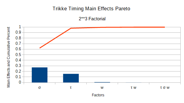
Punch has the greatest effect. In terms of trikke mechanics, quicker turning drives Caster and increases the time Jet can be applied. Punch is further discussed below in Varying Punch.
Cycle has about half the effect of Punch. A shorter cycle allows less time for Jet and encourages quicker Punch. What shorter cycles mainly do for the normal senario is it shortens the time the rider has to Sling and Lean. This increases their push impulses, which translates into more push acceleration.
Mass w doesn't seem to have any effect, not even a small one. One would naturally expect Mass to increase Trikke performance as w increases since the physics of Sling shows a direct relationship. There is no evidence of that effect here. Being somewhat unconvinced, a serial variability experiment is performed below as well; Effect of Rider Weight on Speed.
Coded Multilinear Model
As in the above Full 2**5 Design, a coded multilinear model is easily produced from the effect coefficients being careful to reverse each sign in this case; see Figure 20.
vt = 4.7732125 - 0.1567625 τ - 0.2715875 σ - 0.0069875 w + 0.0356375 τ σ - 0.0016125 τ w + 0.0025625 σ w - 0.0006625 τ σ w
How do we know if the coded multilinear model is any good? Table A-2 in Appendix A shows each of the 8 configurations and the simulation terminal velocity result. It also shows the coded model results and the difference between the sim result and its own; the residuals.
At the bottom, the averages are the same and all of the residuals are zero. The sample standard deviation is therefore zero. So the multilinear model terminal velocity is perfectly determined at the edges of the extreme value range.
Does this hold for interior points? Pick the center point with all codes set to zero. According to the model, the resulting terminal velocity should be the average of all simulation results; 4.7732125 m/s. The factor values for this "center" point case are derived from Table 4:
Center point factor values:
w = 75 kg, θ = 30°, γ = 15°, ψx = -0.675 m, ψy = 0.25 m, aσρ = 2.86 m/s2, v0 = 0 m/s, τ = 1.5, σ = 0.25, φ = 0
with vt = 4.6652 m/s.
This value is not that different from the expected value of 4.7732125 m/s. The model seems to hold in the Factor range interior up to a decimeter per second, less than 2.5% error. Determination of a confidence interval would require error propagation in the simulation. The true relation, however, might be linear or close to it.
Simulated Coasting vs. Measurement
In this article, the simulated coasting results are compared with those in the [calibrated] friction analysis measurements.
Table 6 below shows initial velocity linear coasting scenarios matching those in Table A.7: Simulation vs. Theory in the friction [calibration] study. A second set shows the same scenarios steered 15° tracing a circle. Coasting in a circle evaluates bias due to the simulation processes triggered by a finite turn radius. All scenarios were run with 1.5 second Cycle, Punch at 0.3, Mass at 70 kg and Rest at 0. This experiment like all the others used a time-step of 0.01 seconds. Other time-steps produce similar results, but larger steps produce larger residual standard deviation in the comparison.
Constant Factor values: w = 70 kg, τ = 1.5 s, σ = 0.3, φ = 0.
| Designation | θ (°) | γ (°) | ψx (m) | ψy(m) | aσρ (m/s) | v0 (m/s) | Stop Condition |
|---|---|---|---|---|---|---|---|
| Coast | 0 | 0 | -0.5 | 0 | 0 | 1 2 3 4 5 | v = 0 or 20 cycles |
| Turn Coast | 15* | 0 | -0.5 | 0 | 0 | 1 2 3 4 5 | v = 0 or 20 cycles |
* Unlike the usual limits sweep, once turned to this angle, steering is frozen.
Results for the linear scenarios are presented in Table A-3 Linear Coasting Verification Results in Appendix A. The steered results appear separately in Table A-4 Turn Coasting Verification Results in Appendix A.
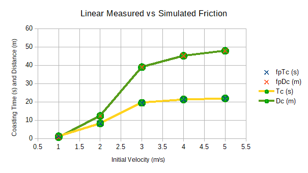
Linear coasting results, Table A-3 and Figure 21, indicate coasting times match to less than a tenth of a second and coasting distances less than 10 centimeters. At the scale of the experiment the measured "X"s on the plot appear to be centered on the simulation value dots. It is worth remembering that only the end points of the experimental runs were measured, where as the simulation provides many points in between. One simulation run could have been used to match all the experimental data, but the points in between wouldn't perfectly match the initial conditions. Interpolation would result in more error. In the figure, the prefix "fp" indicates "friction paper" for the measured coasting times Tc and coasting distance Dc.

Steered coasting results appear in Table A-4 and Figure 22. Turning procedures in the simulation introduce about 3 times more error than the linear runs. Coasting times match to less than a third of a second and coasting distances less than a third of a meter. The measured "X"s and simulated dots still look concentrically centered in the plot on the right. The prefix "fp" indicates "friction paper" for the measured coasting times Tc and coasting distance Dc.
In both the linear and the turned coasting series, the residual standard deviations are less than the residual averages. This means the average simulation results trend away from the actual measurements, being just slightly optimistic and usually less than 1%. These are good results, indicating that the friction behavior is about as reasonable as the measured behavior.
Single Factor Cruising
From a Stop: Each locomotion factor was run separately at an extreme value in an otherwise neutral configuration from a stop. These are designated Steer Only, Camber Only, Sling Only, Lean Only and Jet Only. Steer Only was configuration 0 of the 2**5 DoE Experiment. None of these produced sustained forward motion, so no table is presented here. Many produced traces similar to Figure 14 above. This was no surprise, previous results showed how important steering is to Trikke locomotion. Each of the factors is naturally limited except jet.
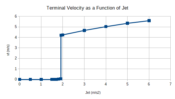
Caster Jet, with Jet the only unlimited input factor, has a critical point. With 30° of steering coordinated with 15° of camber from side-to-side jet only produces at most 0.058 m/s forward motion up through a jet of 1.44 m/s2. At 1.45 m/s2, however, this Caster Jet configuration takes off to a terminal velocity of 4.219 m/s. This critical value changes when the steering limits, Cycle, Punch, Rest and perhaps other factors change. More jet is required at higher steering angles.
Cruise gives each factor a chance to show its worth in the table below. Scenarios with Cruise set near the lowest friction value were run. This means starting each run at an initial cruise velocity of 2.2 m/s. Steer Cruise was configuration 16 in the 2**5 DoE study above, so its resulting dataset was not generated again. The others along with the neutral linear coasting control run are cataloged in Table 7 along with the coasting result used as a control.
Constant Factor values: w = 70 kg, τ = 1.5 s, σ = 0.3, φ = 0.
| Designation | θ (°) | γ (°) | ψx (m) | ψy(m) | aσρ (m/s2) | v0 (m/s)(mph) | Stop Condition |
|---|---|---|---|---|---|---|---|
| Base Line Coast (control) | 0 | 0 | -0.5 | 0 | 0 | 2.2 (4.9) | v = 0 or 20 cycles |
| Steer Cruise | 30 | 0 | -0.5 | 0 | 0 | 2.2 (4.9) | v = 0 or 20 cycles |
| Camber Cruise | 0 | 15 | -0.5 | 0 | 0 | 2.2 (4.9) | v = 0 or 20 cycles |
| Sling Cruise | 0 | 0 | -0.675 | 0 | 0 | 2.2 (4.9) | v = 0 or 20 cycles |
| Lean Cruise | 0 | 0 | -0.5 | 0.25 | 0 | 2.2 (4.9) | v = 0 or 20 cycles |
| Lean Turn Cruise | 15* | 0 | -0.5 | 0.25 | 0 | 2.2 (4.9) | v = 0 or 20 cycles |
| Jet Cruise | 0 | 0 | -0.5 | 0 | 2.86 | 2.2 (4.9) | v = 0 or 20 cycles |
| Jet Turn Cruise | 15* | 0 | -0.5 | 0 | 2.86 | 2.2 (4.9) | v = 0 or 20 cycles |
* Unlike the usual limits sweep, once turned to this angle, steering is frozen.
Results from the single factor cruise runs are compared to the 2.2 m/s neutral coasting configuration; Base Line Coast.
| Residuals | |||||
|---|---|---|---|---|---|
| Designation | Tc (s) | Dc (m) | Final Speed (m/s) | ΔTc (s) | ΔDc (m) |
| Base Line Coast (control) | 11.85 | 19.9074 | 0 | N/A | N/A |
| Steer Cruise | 16.72 | 29.2447 | 0 | 4.87 | 9.3373 |
| Camber Cruise | 11.85 | 19.9458 | 0 | 0 | 0.0384 |
| Sling Cruise | 11.85 | 19.9671 | 0 | 0 | 0.0597 |
| Lean Cruise | 11.85 | 21.8746 | 0 | 0 | 1.9672 |
| Lean Turn Cruise | 13.73 | 26.4128 | 0 | 1.88 | 6.5054 |
| Jet Cruise | 11.85 | 19.9074 | 0 | 0 | 0 |
| Jet Turn Cruise | 10.46 | 20.8605 | 0 | -1.39 | 0.9531 |
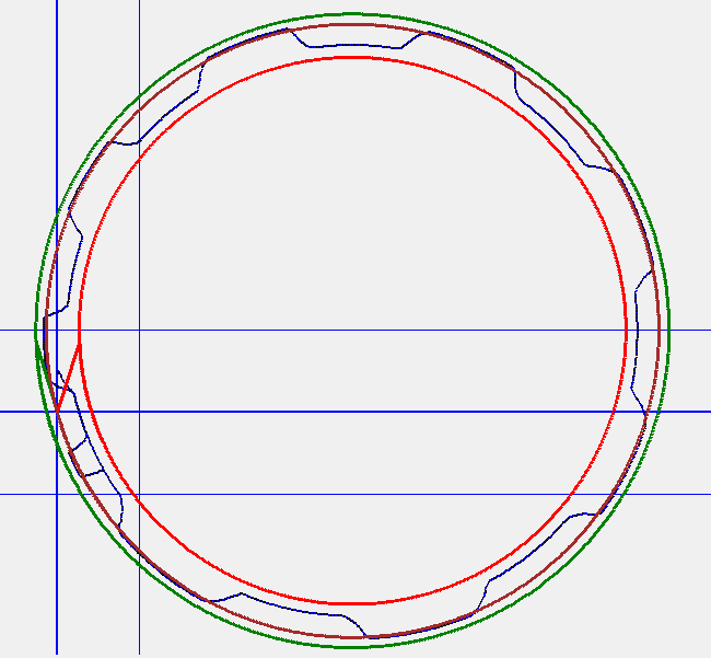
Table 8 shows the residuals of the coasting runs. All of the trials coasted to a stop, but some managed to move farther than Base Line Coast. Steer Cruise gained the most time and ground, over 4 seconds and 9 meters. A 47% improvement from steering while coasting. That invoked Caster to keep the velocity up a little to cover more distance. Lean Turn Cruise managed an extra 2 seconds and 6 and a half meters. In a turn, Lean aligned to the inside of the turn to push the Trikke and rider a few more meters. Lean Cruise added 2 meters to its path over the same time. Jet Turn Cruise added a meter a second faster.
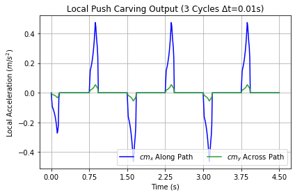
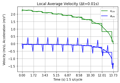
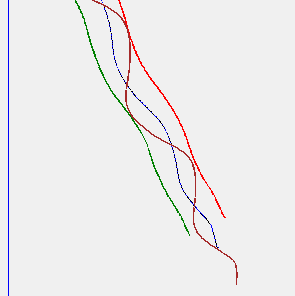
Lean Turn Cruise plotted in Figure 23, shows the shifting blue center of mass trajectory. The brown guide-wheel path, green right wheel and red left wheel paths form concentric circles. It performed quite a bit better than Lean Cruise. In a turn, leaning to the outside causes a push that aligns briefly with the guide-wheel path toward the inside of the turn providing a little incentive to keep the speed up. On the other hand, leaning to the inside causes a slightly lower pull. Below, Figure 25 shows the Lean Turn Cruise carving direct-push output spikes for the first three cycles for leans first to the left then to the right side, the outside of the turn. The full acceleration and velocity profile in Figure 26 shows the same two opposing spikes per cycle in the acceleration. The flat lines are cycle averages. Lean Cruise with no turn simply dumps its energy at right angles to the path. Changes in non-linear friction distribution may account for the small additional distance with Lean Cruise.
Jet Turn Cruise doesn't involve push. Hemijetting to the inside of the turn (turning to the left) applies its full force to the guide-wheel path while hemijetting to the outside decellerates about the same amount. Figure 28 shows that the ride ended when a decelerating right jet forced the speed to zero. While the physics and geometry of jetting against a turn indicate that the Trikke-Rider System decelerates as in the simulation, attempting this on a real Trikke doesn't seem to result in deceleration. It is possible to jet backward, but does not happen easily. A rider has to learn entirely new skill and timing. Steer Jet Cruise achieved a greater terminal velocity firing productively on both hemijets in the 2**5 DoE study of Table 3. In Figure 23 and Figure 24, cruise begins at the intersection of the heavier blue lines. Locomotion continues down the left side, once around and Figure 23 ends in the bottom-right quadrant of the plot.
|
|
|

|
Steer Cruise actually causes the perceived cruise distance to shorten as the limiting angle increases sinusoidal motion as in Figure 1. However, the simulation measures the distance along the winding trajectory of the center of mass. As the stem turns, the center of mass migrates slightly toward the outside of the turn as seen in Figure 27; the blue line. This is a much weaker lean than the previous scenario examined and produces the small amount of caster that accounts for this result. This run covers about 10 cycles. So the distance gained is about nine-tenths of a meter per cycle; nearly one half of a meter per turn!
Effect of Steering on Carving
When starting out from a stop, most Trikke riders begin with wide turns and narrow them only after they get some speed. This experiment looks at how the steering limit angle θ affects caster carve from a stop. 45° was selected as the high limit since larger angles send more velocity across the path than forward along it. An angle of 90° would produce no forward motion at all, except while turning to that limit.
Swath is the distance between the outer edges of the Trikke guide-wheel trajectory during a cycle. The left and right trailing wheels tend to remain inside the swath except when the speed and turn limit is low. Trailing wheels of a Trikke T78 track about 0.5 meters wide. If the combination of cycle time, velocity and turn angle create a smaller swath, a trailing wheel may unexpectedly edge off a rasied path or scrape a wall. Usually, a Trikke rider can count on the trailing wheels falling inside the swath, so there are no sudden surprises.
Using the Normal configuration for Caster Carve factor values, steering angle is varied from 7.5° to 45°. Table 9 presents the results.
Constant Factor values:
w = 70 kg, γ = 15°, ψx = -0.675 m, ψy = 0.25 m, aσρ = 2.86 m/s2, v0 = 0 m/s, τ = 1.5 s, σ = 0.3, φ = 0
| θ rad (°) | Tt (s) | Dt (m) | vt (m/s) | Swath (m) |
|---|---|---|---|---|
| 0.1309 (7.5) | 13.5 | 56.7483 | 4.6900 | 0.550 |
| 0.2618 (15) | 13.5 | 56.0316 | 4.6713 | 1.120 |
| 0.3927 (22.5) | 13.5 | 55.1024 | 4.6460 | 1.665 |
| 0.5236 (30) | 13.5 | 53.6917 | 4.6090 | 2.294 |
| 0.6545 (37.5) | 13.5 | 51.9743 | 4.5716 | 2.865 |
| 0.7854 (45) | 13.5 | 50.0504 | 4.5471 | 3.390 |
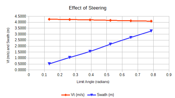
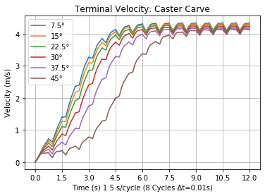
Results: Because terminal velocity vt is a cycle average, the time to achieve it Tt falls on a cycle boundary. The distance it took to reach terminal velocity Dt may actually be a little longer because it too traveled to a cycle boundary time. Swath doesn't change much in the cycles prior to terminal velocity. Figure 29 shows graphs of the terminal velocity and swath over the steering angle limit range. They both appear very linear. Each steering limit and its progress to terminal velocity is plotted in Figure 30. Terminal velocity oscillates around an average for the cycle. This typical behavior is why terminal velocity is determined by the cycle average.
|
|
Another question the simulation data generated by this experiment may shed some light on is this:
How do the energy profiles change with angle?
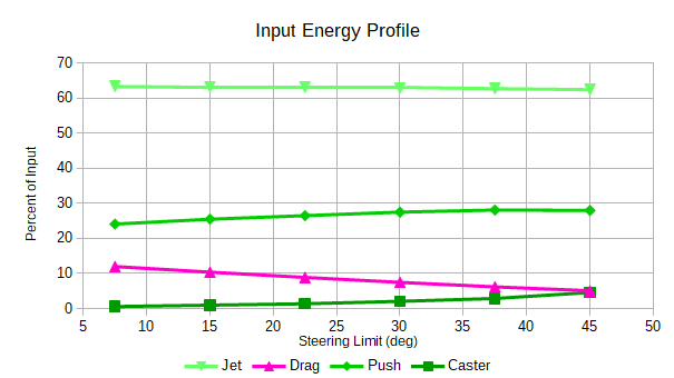
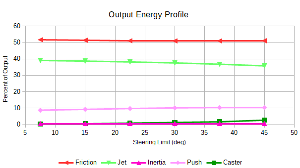
Simulated input energy shown in Figure 31 divides into source categories : Jet, Drag, Push and Caster. Output in Figure 32 partitions into Friction, Jet, Inertia, Push and Caster. Most of these sources are computed as velocity deltas with appropriate translated masses transformed to kinetic energy. Inertia and Friction are transformed to a velocity "equivalent" to integrate into the system velocity. For Friction, the equivalent, comparable velocity is the amount that the gross velocity was reduced because of friction. See the [simulation] paper for details on this topic. Friction work over step duration is its energy contribution. All energy contributions are based on averages over a cycle at terminal velocity and are expressed as percent of total energy.
|
|
Results in this steering limit range are fairly linear. Figure 31 shows that Jet is slightly less effective at higher steering angles because Push and Caster become slightly more effective. Input lost to radial drag decreases with higher steering angle according to Figure 31, but output consumed by friction remains fairly constnt at 50%. On a practical level, these changes in output are not that great. A rider would probably not notice the difference, except overall input energy inceases and output decreases with increasing Steer angles as shown in Figure 33.
Jetting to Attain a Specific Speed
As mentioned above in the discussion of Input Limits, Jet aσρ is one of the more subjective factors. Most of the other inputs are constrained by natural limits, but attainable Jet velocities depend on the rider. Never-the-less, it is possible to discover how much jet is needed to attain terminal velocities in the context of other factor settings. Again the Normal configuration is invoked to provide a basis for the settings of an experiment.
Constant Factor values:
w = 70 kg, θ = 30°, γ = 15°, ψx = -0.675 m, ψy = 0.25 m, v0 = 0 m/s, τ = 1.5 s, σ = 0.3, φ = 0
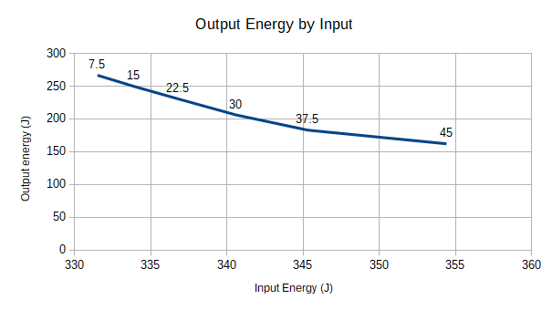
In particular, what are the values of the jet factor that produce a range of operational speeds with "normal" Caster and Carve. Again using the Normal Caster Carve factor values, Jet is explored in the range from 0 to 6 m/s2 to discover their corresponding terminal velocities. It is not contended that all of these Jet values are humanly achievable. The results are presented numerically below in Table 10 and plotted in Figure 34.
|
|
Note that the Jet intervals near the "jump" or "gap" have higher decimal precision in Table 10. The original set of regular Jet values was expanded to include exploring the jump point. Both the upper and lower branch seem to be fairly linear right out to the jump. They don't curve into it even at a tenth of a millimeter per second (data not provided). This graph is typical of a process with a "splitting" factor that operates independently of Jet and terminal velocity. Lower the splitting factor enough and the jump goes away. With short impulsive movements, the lower branch in Figure 34 rises slightly from 0 m/s. The higher, robust carving branch has a pretty good linear model equation with a Pearson Product Moment near 1.
Jet speed is defined to be the forward path component of velocity at the guide-wheel contact point provided by rider generated z-axis rotation. It says nothing about how that rotation is generated by the rider. In the simulation, it is input as a constant, forward path acceleration.
In the context of the other factors held constant, 1.91 m/s2 marks a Jet acceleration threshold that must be crossed to engage the benefit of jetting. If a rider does not provide enough acceleration it is as if no attempt was made to jet. In light of the Trikke [Calibrated] friction model, the jump occurs because it is all too easy to accelerate across the lower friction region. Since the data shows that a jetting threshold must be crossed, how are terminal speeds between 0 and 4.2 m/s (9.4 mph) achieved?
Table 3 configurations 19 through 23 show vts reaching speeds between 2.7 and 2.9 m/s without Jet. They employ Steer, Sling or Push separately or in combination at some Cruise speed. Also, in velocity profiles with Jet like Figure 29, there is continuous velocity increase through the gap for the first few cycles. Once any of these gap speeds has been reached, coasting followed by continued jetting over the threshold should produce a robust average "gap" velocity over the coasting-jetting repetitions. In general, gap velocities are possible to maintain by including periodic Coasting over a couple of cycles.
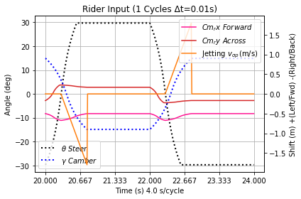
However, Playing with different configurations including Rest φ, terminal velocity continues to jump with a narrowing gap as Cycle increases. The critical value of Jet at the jump also rises. The effective splitting factor appears to be a combination of Rest and Coast with Cycle. Here is one example of a configuration with a terminal velocity in the "gap" of Table 10 by adjusting Cycle, Rest, Punch and Jet. Lowering terminal velocity into the gap using a uniform cycle approach like this involves a trade-off: enough velocity must be maintained early on to get to the lower values of friction, but not so much as to accelerate through them too quickly.
Factor values:
w = 70 kg, θ = 30°, γ = 15°, ψx = -0.675 m, ψy = 0.25 m, aσρ = 3.6 m/s2, v0 = 0 m/s, τ = 4 s, σ = 0.15, φ = 0.3
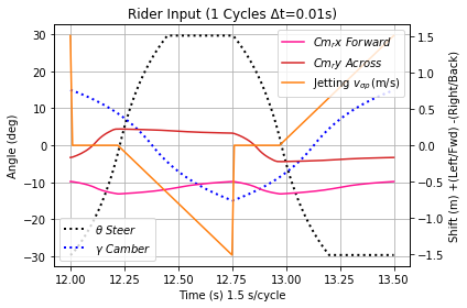
This configuration has a four second cycle-time, during which the rider rests 60% of the time, see the robot-rider input in Figure 35. Jet accelerates at 3.6 m/s2 for 0.8 seconds ramping the guide-wheel to an additional 1.848 m/s, about the same as Push, which contributed half as much to the output energy. Its simulated terminal velocity reaches 3.7384 m/s, which is in the upper part of the previous gap discussed.
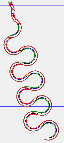
The Swath of its path in Figure 36 begins quite small, 0.8 m, as the rider struggles to overcome friction. Once the system begins to accelerate down the friction curve, the swath opens to a whopping 7.0 m because the loops fold back and forth over its 66.75 m guide-wheel path. The Trikke actually travels a little upstream just before turning the other way. Along the path, this Trikke cracks 8 mph, but a bystander probably perceives the Trikke traveling at the "swath speed"; the speed at which the swath moves forward. From the starting point, the swath length is about 28 m. 28 m traversed in 24 seconds is only 1.1667 m/s. That doesn't help with finding "mid-gap" configurations much, but it illustrates that there are various ways to measure the speed of a Trikke!
|
|
|
Varying Punch
What about Punch? Does punching really help? Punch had the greatest effect on terminal velocity of the three factors measured in the DoE Full 2**3 Factorial Design with Cycle, Punch and Mass experiment. In this experiment, Cycle and Mass are kept constant and Punch is varied over five values from a tenth of a hemi-cycle to half. Again, Normal Caster Carve is the configuration of choice for setting the constant factor values.
Constant Factor values:
w = 70 kg, θ = 30°, γ = 15°, ψx = -0.85 m, ψy = 0.25 m, aσρ = 2 m/s2, v0 = 0 m/s, τ = 1.5 s, φ = 0.
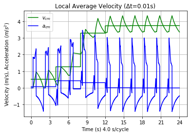
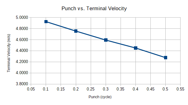
Table 11 presents the results for Punching from a stop. Because terminal velocity detection occurs on cycle boundaries, the time and distance to vt is on average half a cycle farther than it might really be. The terminal velocities are plotted in Figure 38. Amazingly, they appear to be linearly related. Increasing Punch, the time it takes to turn from one direction to the other, slows the Trikke-Rider System 0.65 m/s for the Normal configuration.
|
|
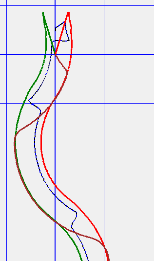
Punching quickly at σ = 0.1 cycles, results in double the Normal output Caster energy, only about half the Normal output Push energy and increases Jet output by a seventh. Figure 39 portrays the starting trajectories of the TRS center of mass (blue), the guide-wheel (brown) and left (red) and right (green) wheels. Because the rider is more massive than the Trikke, the center of mass of the whole system follows that of the rider to a couple of centimeters. The rider's Sling and Lean effects can be clearly seen. The red and green "V" is due to the outer wheel turning inward then back as the rider twists the trikke in its first turns. Once the guide wheel grips the road, all the wheels advance in a signature Trikke wave pattern. Each blue line segment is a meter apart.
|
|
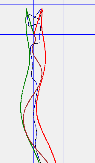
Punching slowly at σ = 0.5 cycles, results in a little less Normal output Caster energy, about one and a half the Normal output Push energy and decreases Jet output by a quarter. Figure 40 portrays the starting trajectories of this configuration. Again, the red and green "V" is due to the outer wheel turning inward then back as the rider twists the trikke in its first turns. It takes a couple more cycles to get moving as witnessed by the short initial, snakey guide-wheel turns (brown). Lean lines across the path are initially just as close as those for σ = 0.1 in Figure 39, but remain closer even though the there is equal time between them. Steering less aggressively makes it more difficult to overcome friction. Notice that even though the guide-wheel snakes a bit at first, the rear wheels do not show such small-scale turning.
Figure 41 shows carve push output measuring about 3.7 m/s2 for σ = 0.1, while Figure 39 for σ = 0.5 shows output at 1.4 m/s2 with spikes five times as wide in time. Carving jet acceleration was the same for all configurations in this experiment, but because steering was short, σ = 0.1 built up Jet speed to 2 m/s, while 0.5 only mustered 1.2 m/s.
|
|
Caster is at its prime during the quick turns of σ = 0.1, providing increased force with added guide-wheel velocity over 1.5 m/s for a very short time in Figure 43. Figure 44 for σ = 0.5 has spikes only a tenth of that magnitude, but 5 times wider. Never-the-less, the total increase amounts to only 5% velocity increase for σ = 0.1. It appears Punch operates mostly by allowing more time in a cycle to Jet.
|
|
As increased Jet accelerates the Trikke with σ = 0.1, friction decreases as the Trikke approaches the 2.2 m/s minimum friction point allowing it to accelerate to the other side of the friction "well" where it is limited by a terminal velocity. Figure 45 shows path friction evaporating about during the first cycle. The story is quite the opposite for σ = 0.5 in Figure 46. Initial velocity gains are much smaller, keeping friction high during the first cycle.
|
|
Effect of Rider Weight on Speed
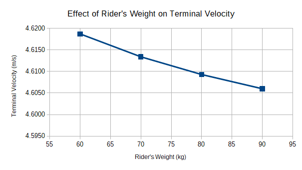
A main feature of Trikke locomotion entails flinging the Trikke forward into the guide-wheel path. It seems likely that the higher the ratio between the rider's weight and that of the Trikke, the more forward motion can be generated. Therefore, on average, heavier men should be able to carve faster than lighter women. What does the simulation indicate?
Configurations for varying rider weight use Normal Caster Carve as the base configuration. For the reasons cited above in the article on Cycle, Punch and Rider Mass Factors, some good values for Mass are 60, 70, 80 and 90 kg.
Constant Factor values:
θ = 30°, γ = 15°, ψx = -0.675 m, ψy = 0.25 m, aσρ = 2.86 m/s2, v0 = 0 m/s, τ = 1.5 s, σ = 0.3, φ = 0
The results are presented numerically below in Table 13 and plotted in Figure 47.
|
|
These results indicate that the dynamic processes in the system have not biased the generation of speed based on weight. The difference between the high terminal velocity and the lowest one is only about a centimeter per second. Providing lighter riders can generate the same Jet velocities as heavier ones, what could the equalizing physics be? To generate Jet, the rider must rotate their body, overcoming rotational inertia to transfer rotation to the Trikke. While the Trikke's moment of inertia is the same for both riders, the lighter one has less bodily moment around the vertical axis. The simulation does not account for this in generating the Jet, but it does figure into the system rotation around the vertical axis. Therefore, it is easier for the system as a whole to rotate faster for the light rider's Jet.
Some of the other data collected during the experiment is compared in Table 14 below. Light refers the 60 kg configuration, while Heavy refers to the 90 kg configuration.
Rotational inertia is indeed lower for the lighter rider. Examine Figure 45 the carving rotation mechanism graph for the lighter rider. The "Base" rotational inertia is the low part of the stem inertia Iσtc (black) and Extended-Trikke IEtc (orange) curves during the part of the cycle where the turn-radius is lowest - where steering is at one of its limits. During the turn as the turn-radius increases to infinity, so does the rotational inertia of the system since it is translated to the turn-center via the Parallel Axis Theorem. The graph cuts off the spike so the base values can be seen. The green and blue curves trace technical internal variables discussed in the [Physics] paper. Looking at the base values, the light rider has rotational inertia that's 1/4 less than for the heavier rider in Table 14.
Friction must also favor the lighter rider, simply because the load on each axle is less. Indeed, the data shows the terminal cycle average total friction for the light rider is about 300 and 485 N for the heavy rider.
In previous experiments presented in this account, Jet was seen to affect locomotion much more than carving direct-push, where Sling and Lean enter the calculation. As mentioned above, push is directly dependent on the ratio of the rider and Trikkes' weights. Here, the light rider pushed with velocities about 7% short of the heavy rider.
For the lighter rider, the effect of rotational inertia increases the effectiveness of Jet, friction resists less, and the weight ratio decreases the contribution of push resulting in a stalemate with regard to speed.
Conclusion
What makes a Trikke go? This study is an attempt to understand the basic mechanisms that drive a Trikke by running qualitative and quantitative simulations of Trikke locomotion. Calibration of the friction model via empirical coasting trials and terminal velocities allow this Trikke simulation to be quantitatively believable and behaviorally accurate. A key to obtaining some of the results involved tuning the digital robot to drive the Trikke in a manner similar to an experienced rider. Synchronization of robot actions and the phases of their critical points required several attempts. It is one thing to coordiante a good ride, it is another to know how you are doing it. All attempted robot configurations succeeded in driving the Trikke. The best one, presented in [simulation] also seems to mimic one of my fastest riding styles. Peering into the nuances of these mechanisms working together through these virtual experiments has verified some experiential insights, changed the author's opinions on others and produced a few new ones. More behavior awaits exploration via simulations like this, especially Trikke design, but this study provides much to think about in terms of exposing and improving riding technique.
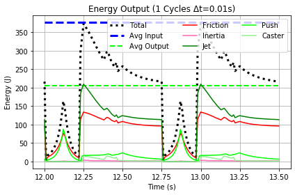
For best sustained locomotion of a Trikke, the simulation experiments suggest starting turns with a guided Push into the guide-wheel path, followed by maximum Jet and minimal steering at speed. Starting out really is the hardest part of ride! Yet, the experiments indicate ways to master this when riders coordinate the factors from positions that increase control effectiveness and respond to where they are on the friction curve. In the interest of applying technique at the appropriate point in the cycle, Figure 48 shows how the various components of output energy fluctuate over one cycle at terminal velocity in a Normal Caster Carve configuration. Push (green in the Figure), though not massive, dominates the beginning of the turn and dies out as the guide-wheel passes straight as all jetting impulses must. Caster (light green) and Jet (dark green) kick in past straight as the turn continues to its limit on the other side. Caster only plays a small role and ends as steering stops at its limit. Jet continues until the beginning of the next turn. Push energy following the initial productive Push, is actually Pull, working against forward motion. Its effect is minimized by the rider's center of mass movement on the Trikke in a similar way that the initial Push is maximized by the rider's movement.
At the outset, ten simulation input factors were introduced and named. Configurations in the experiments were designated by combinations of the factor names and some were combined into mechanism names like Caster and Carve. "Extreme" values assigned to each served as code values and constraints on their ranges in the experiments. A "normal" configuration, Normal Caster Carve, served as an example and control for comparing the many experiment outputs.
Factor extreme values formed the basis of four DoE non-replicant designs. A preliminary DoE Factorial 2**(6-2)IV Design screened for the factor with the greatest effect; Steering. No steering = no motion. A Trikke goes only when steered side-to-side with a couple of notable exceptions, like pushing forward followed by a very slow return to forward position.
Effects from the DoE Full 2**5 Design indicated this decreasing effect order for the five factors explored: Jet, Cruise, Lean and Sling tied with Camber. This order might have been different depending on how the robot-rider is configured. It was found that the four other factors detract from Jet. However, there were enough "degenerate" configurations - those that did not exceed 4.9 m/s - that when those factors were added to them, they managed to increase vt enough for each to be considered a positive effect. Unfortunately, the multilinear model did not pass the center point test, so it cannot replace the simulation for factor values inside the extremes used in the experiment.
To complete group Factor analysis, the DoE Full 2**3 Design showed three more factors in descending effect: Punch, Cycle and Mass. Results showed that a rider can speed up the ride by decreasing Punch and Cycle (time). Decreasing Punch increases the Push and Caster impulse, but most importantly gives Jet more time to develop. Surprisingly, the rider's mass had virtually no effect on the ride providing a lighter person can generate the same amount of jet as a heavier one. This time, the multilinear model looks like it could be linear.
Results from Serial Variability Experiments
- Simulated Coasting vs. Measurement verified that the Simulated coasting terminal velocities match those of the empirically [calibrated] friction study pretty well. Turn coasting was still close, but there was some process gain.
- Single Factor Cruising experiment found each factor alone fails to sustain a vt. However, Steer Cruise, Lean Turn Cruise and Lean Cruise prolong coasting to a stop.
- The Effect of Steering on Carving shows that lower steering limits are slightly faster along the path, but have much less Swath than wider turns. Lower steering limit angles also have higher swath speed as their paths are straighter. Swath increased linearly with limit angle. Energy profiles were relatively unchanged. Jet decreased a bit at higher angles, while Caster became slightly more relevant.
- In Jetting to Attain a Specific Speed two vt branches were separated by a 4 m/s jump at just over 1.91 m/s2. This led to exploring how speeds in the gap could be sustained. By alternating cycles of acceleration with coasting, any average cycle speed in the gap can be produced. Producing them with Rest in a single terminal cycle proved practically illusive.
- Varying Punch downward achieves higher vt, linearly. The data shows that Punch operates mostly by increasing the cycle time available to Jet.
- Effect of Rider Weight on Speed also showed rider's mass has virtually no effect. Parsimonious physics keeps things balanced. Though from the data for the 60 kg rider, Figure 49 illustrates how straight the motive vectors pass through the TRS center of mass. Up is forward in the trikke inertial frame. The angles of the orange Jet and black Push velocity rays are those of the TRS center of mass path. 30° is the steering limit, but the TRS center of mass path does not turn so sharply. Each ray originates on the cycle time-line where it was produced. A plot of the stem's turn angle θ is imposed on the graph for reference. Note the Push rays below the Jet rays are actually Pull, detracting from forward progress, but greatly over-powered by Jet.
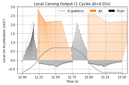
Perhaps the most structured finding pertains to mechanism limits producing speed. Table 15 below shows various speed ranges and the mechanism or technique needed to produce it. As noted above in Jetting to Attain a Specific Speed, these ranges change with Cycle-time, Punch and Rest. The table applies to a base configuration of Normal Carve Cruise used in many of these experiments.
| Speed and Critical Value | Indication of Technique |
|---|---|
| vt > 0 m/s | Carving with weak Jet |
| vt > 0.06 m/s | No indication this range is achievable on flat ground w/o wind |
| vt > 2.2 m/s | Combinations of factors starting with Cruise over 2.2 m/s, but no Jet |
| vt > 3 m/s | Combination of Carving alternating with Coast and/or possibly Rest |
| vt > 4.2 m/s | Carving with Jet > 1.86 m/s2 |
Note the difference between input and output energy accounting indicates that much of the energy entering the Trikke-Rider System is consumed internally to create output as in Figure 48. Never-the-less, this efficiency over 50% seems high compared to the disscussion related to Figure 6 about Terminal Output Energy Profile. This includes mechanical transfer of Jet that varies between 100% and about 75% every cycle, the radial Push component that can swallow almost all Push action depending on the momentary steering angle and all of Caster if the rider fails to supply the action it requires - and it has been assumed that happens. However, it seems that is not enough to account for the entire gap.
As these simulated experiments were performed, a couple of bugs were found in the program and corrected. Affected experiments were rerun. The worst bug discovered related to Punch changes resulting in less Sling from the robot rider.
Appendix A: Result Tables
Glossary
Camber, cambering Wheel tilt angle from vertical rotated around a wheel's forward path direction. Tilting a Trikke's steering column serving as the Camber-Lever to the left or right side creates a nearly equivalent vertical tilt in all three wheels. Foot-deck tops also angle synergistically to increase grip in a turn. For Trikkes, cambering generally refers to tilting the steering column from side-to-side coordinated with steering. Cambering enhances the effects of carving and castering.
Camber-Lever A second-class lever of the stem with fulcrum on the road and action from cambering that moves the yoke. It also interacts with the two levers involved in castering.
Camber thrust When a cambered wheel rotates, tread-particle elliptical trajectories are constrained to run straight when contacting the ground. This asymmetry causes a change in their momentum (a force) at right angles to the inside of the camber angle. This force and increasing change in camber pull the wheels into the turn avoiding dangerous wheel slips to the outside.
Carve, carving Most dictionaries don't define a sports sense of this word! [sportsdefinitions.com] does for skiing and skateboarding, basically a turn accomplished by leaning to the side and digging an edge or wheel into the path. In the case of "carving vehicles" or "CV"s, carving is a transfer of momentum from the rider to the vehicle synergistically constrained by ground forces on the wheels. The Trikke seems best engineered to claim this action as a primary form of locomotion. This motion mechanism provides action to the guide-wheel contact point around the Turn-Lever.
Caster, castering Most dictionaries don't define a sense of this word as a verb! Here, it is defined as a form of locomotion. To caster is to move by quickly turning a wheel with positive caster and positive trail back and forth to produce forward motion. The offset contact patch causes the vehicle frame head or yoke to move sideways a couple of inches pulling part of the vehicle's trailer mass into the turn. Impulse created by this motion in the direction of the drive wheel path first pulls, then pushes on the vehicle's stem assembly. It is the sideways rotation not the stem pull or push that creates a small jetting impulse. This appears to be the primary means of locomotion for the [EzyRoller], [Flicker], [PlasmaCar] and Wiggle Ride-On Car by Lil' Rider (no web presence) rider toys and one of the modes for a Trikke. Two levers mechanize this motion: the Yoke-Lever and the Trailer-Lever.
Caster angle - positive, negative The angle a steering column makes with the road. It is positive when the angle slopes up toward the back of a vehicle. It is negative otherwise.
Caster pull When the handlebars of a Trikke are turned and tilted quickly toward the center, the geometry of the steering mechanism and constraints on wheel motion, throws the yoke into the turn up to a few inches and pulls the Trikke's Extended-Stem and trailer a quarter inch or so closer together in a fraction of a second. Though the rotation is small, most of the weight of the Trikke and its rider get spun around the transom. The pull generates no immediate jetting impulse. Steering resistance increases as caster pull builds local angular momentum.
Caster-push When the handlebars of a Trikke are turned and tilted quickly away from the center, the geometry of the steering mechanism and constraints on wheel motion, throws the yoke into the turn up to a few inches and pushes the Trikke's Extended-Stem and trailer a quarter inch or so apart in a fraction of a second. As the turn reaches its limit, the built up angular momentum transforms into a jetting impulse. The rider synergistically leverages this push for speed by synchronizing carving impulses with it.
Citizen scientist An individual who voluntarily contributes time, effort, and resources toward scientific research in collaboration with professional scientists or alone. These individuals don't necessarily have a formal science background. See What is citizen science? [Citizen Science].
Conservative force A force that can be expressed as the gradient of a potential. When this is possible, the work done by the force is not dependent on the path taken. A "round trip" by different paths of the same length requires the same amount of work. Gravity is a familiar conservative force.
Design Of Experiment (DoE) A type of designed experiment contrived to efficiently identify (screen for) the control factors that affect the process being studied the most (main effects). DoE can model and compare the effects of several factors against each other using Yates analysis. It attempts to optimize the differences in effects and minimize the number of trials needed to obtain them. When models are attained they have least-squared, multilinear properties subject to the confounding structure of the experimental factors. When not attained, the true process model is non-linear.
Direct-Push and Pull, slinging Intentional impulse created as the rider quickly moves his or her center of mass in the opposite direction of the handlebars. Lightening the load on the drive wheel and pushing the Trikke forward with arms and legs feels like "slinging" the Trikke forward. In order to retain the ground gained, this maneuver must be concurrent with or followed by steering, cambering or both. During the push or pull, the mechanism produces a jetting impulse; acceleration for the push, deceleration for the pull.
Dynamics Study involving variables related to the generation of an object's motion. Answers questions about how motion is produced.
Equation of motion (EOM) Application of conservation laws or principles like least action and balance of forces and torques to produce global kinematic and other equations for a system. For example, an approach due to Lagrange starts with energy conservation, equivalences between kinetic and potential to derive system velocities, then other kinematic quantities and sometimes Newton's force-based EOMs can be derived for the system. D'Alembert's principle allows various constraints on part velocities and positions to be incorporated in some EOMs. Other approaches create state-based generalized coordinates and use lie algebras to represent system functions. While many EOMs cannot be solved symbolically, they lend themselves to numerical solutions via computer simulation.
Extended-Stem The part of the TRS that is turned by the rider during castering. Composed of the stem, hands and wrists of the rider's body. Does not include body parts considered part of the trailer. In lever systems, one-third of a linkage between two moving parts can be shown to act as if stationary with respect to the closest attachment. So, one-third of a hand and arm acts as if stationary to the stem, another third to the trailer and a third acts with the arm's own momentum.
Extended-Trikke The part of the TRS that slings during carving. Composed of hands, wrists, feet, ankles and parts of the rider's body that sling with the Trikke. The part of the reduced rider's body producing the jetting and Direct-Push impulse is not part of the Extended-Trikke. In lever systems, one-third of a linkage between two moving parts can be shown to act as if stationary with respect to the closest attachment. So, one-third of a foot and lower leg acts as if stationary to the deck, another third to the rider and a third acts with the lower leg's own momentum.
GCF Global Coordinate Frame, "lab" or "observer's" frame may contain an infinite number of LCFs twisting, moving and even changing size everywhere. The Trikke-Rider System LCF is fairly well behaved inside the GCF; it has a common z-axis and doesn't change scale. Observers can see and measure the TRS as it moves and turns and can all obtain the same values. But they can't feel the accelerations of the Trikke like the rider.
Jetting, hemijet The angular component of carving. Beyond the "natural" body twist accompanying slinging, the rider extends the foot outside the turn by lowering his center of mass, leaning back and twisting the hips into the turn. This angular impulse adds angular momentum to the system via the Parallel Axis Theorem through rotation about the TRS center of mass. The word comes from an outdated skiing technique using both feet. Technically, this is "alternating hemijetting" since each foot independently executes half of a "jet" (a hemijet) in one drive-cycle. However, it is possible to jet with both feet.
Kinematics Study involving variables related to the classification and tracking of an object's movement. Answers questions about the form and characterization of motion, not how the motion is produced.
Lateral plane An imaginary plane that separates the front half of an object from its back half. Its normal is parallel to the front-to-back axis of the object.
LCF Local Coordinate Frame, inertial frame or just local frame is the rider's world where the Trikke and everything on it seems relatively stationary compared to the rest of the world. It is "inertial" because the Trikke and rider "feel" centripetal force in a turn and the accelerations of its movement. Yet the Trikke remains close to the rider. "Forward" is pretty much ahead. There is a wheel always under the left foot. Things are local and for the most part in their expected places. When the rider measures things relative to his locality in the GCF, they are usually different than the same things measure by observers in the GFC.
MA, Mechanical Advantage A ratio, percentage or number expressing the force multiplier or efficiency of a lever system. For simple levers, it is the distance of the action to the fulcrum divided by the distance of the load to the fulcrum.
Nonholonomic system (also anholonomic) In physics and mathematics a nonholonomic system is a type of system that ends up in a different state depending on the "path" it takes. In the case of the Trikke, frictional forces and some geometric constraints restricting velocity but not position prevent the system from being represented by a conservative potential function. It is "non-integrable" and not likely to have a closed-form solution.
Normal A "normal" to a plane, is a ray starting at the plane which is at right angles to every ray in the plane that starts at the intersection point. Notice that the normal cannot lie in the plane. Its unit direction is also the "direction" or "orientation" of the plane.
Parallel Axis Theorem One of two theorems by this name. Translates a moment of inertia (moi) tied to a center of mass and rotation axis to an offset but parallel axis. If the moi is expressed as a tensor with no particular rotation axis, then it translates to an arbitrary point, usually on the object. The second namesake does the same for an angular momentum vector. There is also a theorem called the "Second Parallel Axis Theorem" which is simpler to apply in some contexts.
Reduced rider About fifteen percent of the rider's body mass acts as if it is a part of the Trikke. Hands and wrists move largely in unison with respect to the handlebars. Corresponding parts of the legs act as if part of the decks on the arms of the Trikke. This "reduces" the effective mass and distribution of the rider, while increasing that of the Extended-Trikke and Extended-Stem.
Sagittal plane An imaginary plane that separates the left half of an object from its right half. Its normal is parallel to the left-right axis of the object.
Steering column, stem The controlling mechanism surrounding the steering axis. Composed of the steering column, handlebars, rider's hands and parts of his forearms (about 1/3) as well as the yoke, front wheel, axle, bearings and attachments. It is considered part of the Extended-Trikke, but is the part of the TRS not included in the trailer. It is also a lever; the Camber-Lever.
Stride A body in motion has linear and rotational (or angular) velocity. Parts of the body have different velocities depending on their distance from the rotation center. Stride is the difference between a part's velocity and the linear velocity of the whole body at its mass center. Rotational velocity can be expressed as a linear velocity, v̅, at right angles to a radius pointing from the rotation center: (v̅ = ω̅ × r̅). When the rotation center is the turn-center of the TRS, and the radius ends at a wheel, the difference between v̅ and the TRS linear velocity is that wheel's stride.
Swath As a Trikke snakes its way along, the outer edges of the wheels trace a wide ribbon-like path down the road. At terminal velocity, if one connects the outer most edges of the wavy ribbon on both sides to get a long rectangle, the width of that outlined area is the "swath" covered by the Trikke. In simpler terms, it is the width of the path covered by the Trikke. If something is within the swath of the Trikke, there's a decent chance it will be hit depending on Trikke's trajectory.
Trailer The parts of a TRS that are rotated around the transom and pulled or pushed slightly by the Trailer-Lever while castering. Consists of the parts of a Trikke other than the steering column, front drive wheel, handlebars, "handlebar-stationary" hands and parts of the forearm (about a third of it).
Trailer-Lever Caster action is applied at the yoke by the Yoke-Lever which rotates it and pulls or pushes it. The center of mass of the trailer is its load. Its fulcrum is the Transom point. The Trailer-Lever is a second-class lever and push-rod.
Transom Used to indicate the point on the line between the rear wheel contact points with the ground acting instantaneously as the Trailer-Lever fulcrum. Its position is determined by the ratio of instantaneous friction at each wheel. Thus, when the load is nearer the left wheel, the transom point, or just transom, is nearer the left wheel. For equal friction on both wheels, it is in the center of the line between contacts.
TRS Trikke-Rider System. Refers to the entirety of the physical system composed of the Trikke, all of its relevant parts and behaviors and the rider with all relevant parts and behaviors needed to complete the current investigation. Though the road, air and other parts of the environment are required to operate the system, they are not considered part of it.
Turn-Center A Trikke orbits this stationary point at a constant radius until the steering angle is changed or a wheel slips. When steering straight, the turn-center is not defined and the turn-radius is considered infinite. Jetting makes use of the turn-ray as a second-class lever acting on the system center of mass.
Turn-Lever A turn-ray is the ray from the turn-center to a point on the Trikke. When the point is the guide-wheel contact point, the ray becomes an important motive lever as all TRS motion must move the contact point around the turn-center.
Yoke Idealized point of intersection for the three structural tubes that characterize a Trikke. This genius articulation is fairly complex and precisely manufactured. It is the soul of the Trikke - if there is one. Constant motion from steering, cambering and road vibration are robustly endured, while keeping all the wheels aligned without toe-under or splaying.
Yoke-Lever Constitutes part of the castering mechanism set in motion by turning the stem. The rotation produces an action at the yoke, which is also the load. Its fulcrum is the guide-wheel contact patch. The movement of this yoke-load acts on the Trailer-Lever which rotates it and pulls or pushes it. The Yoke-Lever is a degenerate lever.
References
Patents
[Trikke Patent] J. Gildo Beleski Jr. Cambering Vehicle and Mechanism. US Patent 6,220,612 B1. Dec 20, 2005. Google Patents  US6976687B2. Prior: 1999 US09434371 Active, 2000 US09708028 Active, 2002 US10331558 Active, 2004-06-25 US10876497 Expired - Fee Related, 2004-11-18 US20040227318A1 Application, 2005-12-20 US6976687B2 Grant.
Control Theory in Robotics
[RoboTrikke] Sachin Chitta, Peng Cheng, E. Frazzoli, V. Kumar. "RoboTrikke: A Novel Undulatory Locomotion System". In Proc. IEEE Int. Conf. Robotics and Automation, pages 1597-1602, Barcelona, Spain, April 2005. DOI: 10.1109/ROBOT.2005.1570342.
[Roller-Racer] P. S. Krishnaprasad and D. P. Tsakiris. "Oscillations, SE(2)-Snakes and Motion Control: A Study of the Roller Racer." Technical report, Center for Dynamics and Control of Smart Structures (CDCSS), University of Maryland, College Park, 1998.
[Roller-Walker] Gen Endo and Shigeo Hirose. "Study on Roller-Walker: Multimode steering control and self-contained locomotion". In Proc. IEEE Int. Conf. Robotics and Automation, pages 2808-2814, San Francisco, April 2000. DOI: 10.1109/ROBOT.2000.846453
Papers
[CarveABike] Sachin Chitta, V. Kumar. "Biking Without Pedaling". November 2006. Chitta, Sachin. “Biking Without Pedaling.” (2006).
[Air Force] Charles E. Clauser, et al., Air Force Systems Command, Wright-Patterson Air Force Base, Ohio. August 1969. Pub AD-710 622.
[Moment Of Inertia] Dr. J. B. Tatum. Chapter 2, 'Moment Of Inertia', section 2.8. University of Victoria. 2017. http://astrowww.phys.uvic.ca/~tatum/classmechs/class2.pdf, 2019.
[physics] Michael Lastufka, "Body-Powered Trikke Physics" June 2020.
[calibrated] Michael Lastufka, "Empirical 2nd Degree Friction Model Solution" June 2020.
[simulation] Michael Lastufka, "Dynamic Model of a Trikke T78 Air" June 2020.
[magic] Michael Lastufka, "Trikke Magic: Leveraging the Invisible" June 2020.
Other
[Trikke] Trikke Tech Inc. 132 Easy St Suite D1, Buellton, CA 93427 – USA. https://www.trikke.com/fitness/, 2019. Email: info@trikke.com
[SB Trikke] South Bay Trikke 707 Fremont St, Las Vegas NV 89101 – USA. https://southbaytrikke.com/support/about/bpv/, 2019. Email: https://southbaytrikke.com/support/contact/
[George Box] Box, George E. P. (1976), "Science and Statistics" (PDF), Journal of the American Statistical Association, 71: 791–799, DOI: 10.1080/01621459.1976.10480949.
[Nonstandard Analysis] MathWorld: Nonstandard Analysishttp://mathworld.wolfram.com/NonstandardAnalysis.html. 2019.
[POV-Ray]http://www.povray.org/, 2019.
[sportsdefinitions.com] SportsDefinitions.com. http://www.sportsdefinitions.com/, 2019.
[EzyRoller] EzyRoller LLC. 22588 Scenic Loop Rd., San Antonio TX 78255 - USA. https://www.ezyroller.com/, 2019. Email: info@ezyroller.com
[Flicker] Yvolution USA Inc. 2200 Amapola Court, Suite: 201, Torrance, CA 90501 – USA. https://yvolution.com/, 2019. Email: support@yvolution.com
[PlasmaCar] PlaSmart Inc. 228-30 Colonnade Road, Nepean, Ontario K2E 7J6 - Canada. https://plasmarttoys.com/, 2019. Customer Service 1-877-289-0730 Ext. 214
[Citizen Science] SciStarter. https://scistarter.com/citizenscience.html, What is citizen science?, 2019. Email: info@scistarter.com
[Weight] Human body weight, Wikipedia https://en.wikipedia.org/wiki/Human_body_weight, 2020.
[gme] Muscle, Wikipedia https://en.wikipedia.org/wiki/Muscle, 2020.